Last updated: 2021-10-19

Checks: 7 0

Knit directory: veg_alcontar/

This reproducible R Markdown analysis was created with workflowr (version 1.6.2). The Checks tab describes the reproducibility checks that were applied when the results were created. The Past versions tab lists the development history.

R Markdown file: up-to-date

Great! Since the R Markdown file has been committed to the Git repository, you know the exact version of the code that produced these results.

Environment: empty

Great job! The global environment was empty. Objects defined in the global environment can affect the analysis in your R Markdown file in unknown ways. For reproduciblity it’s best to always run the code in an empty environment.

Seed: set.seed(20211007)

The command set.seed(20211007) was run prior to running the code in the R Markdown file. Setting a seed ensures that any results that rely on randomness, e.g. subsampling or permutations, are reproducible.

Session information: recorded

Great job! Recording the operating system, R version, and package versions is critical for reproducibility.

Cache: none

Nice! There were no cached chunks for this analysis, so you can be confident that you successfully produced the results during this run.

File paths: relative

Great job! Using relative paths to the files within your workflowr project makes it easier to run your code on other machines.

Repository version: 9e36cbb

Great! You are using Git for version control. Tracking code development and connecting the code version to the results is critical for reproducibility.

The results in this page were generated with repository version 9e36cbb. See the Past versions tab to see a history of the changes made to the R Markdown and HTML files.

Note that you need to be careful to ensure that all relevant files for the analysis have been committed to Git prior to generating the results (you can use wflow_publish or wflow_git_commit). workflowr only checks the R Markdown file, but you know if there are other scripts or data files that it depends on. Below is the status of the Git repository when the results were generated:


Ignored files:
    Ignored:    .Rhistory
    Ignored:    .Rproj.user/

Note that any generated files, e.g. HTML, png, CSS, etc., are not included in this status report because it is ok for generated content to have uncommitted changes.

These are the previous versions of the repository in which changes were made to the R Markdown (analysis/temporal_analysis.Rmd) and HTML (docs/temporal_analysis.html) files. If you’ve configured a remote Git repository (see ?wflow_git_remote), click on the hyperlinks in the table below to view the files as they were in that past version.

File	Version	Author	Date	Message
Rmd	9e36cbb	ajpelu	2021-10-19	add new figures
html	bbd9ef6	ajpelu	2021-10-13	Build site.
Rmd	c80ead3	ajpelu	2021-10-13	wflow_publish(“analysis/temporal_analysis.Rmd”)
html	5300bc8	ajpelu	2021-10-13	Build site.
Rmd	c9913ef	ajpelu	2021-10-13	wflow_publish(“analysis/temporal_analysis.Rmd”)

Introduction

Read data
Rename the levels of zona:
- Pyric herbivorism (HP, from spanish Herbivorismo pírico): old Quemado con pastoreo
- Prescribed Fires (QP, from spanish Quemas Prescritas): old Quemado sin pastoreo

veg_raw <- readxl::read_excel(here::here("data/Datos_congreso_AEET.xlsx")) %>% 
  janitor::clean_names() 

autumn_fire <- lubridate::ymd("2018-12-18")
grazing_start <- lubridate::ymd("2019-10-01")

veg <- veg_raw %>% 
  rename(fecha = fecha_muestreos, 
         shan = i_shannon, 
         consumo = tasa_consumo, 
         riq = riqueza) %>% 
  mutate(treat = as.factor(case_when(
    zona == "Quemado con pastoreo" ~ "HP", 
    TRUE ~ "QP"
  ))) %>% 
  mutate(meses = as.numeric(as.character(lubridate::interval(autumn_fire, lubridate::ymd(fecha)) %/% months(1)))) %>% 
  mutate(quadrat = as.factor(quadrat)) %>% 
  mutate(meses = case_when(
    meses == 0 ~ -1, 
    TRUE ~ meses
  ))

# Subset of data (pre/post) 
ad <- veg %>% filter(meses %in% c(-1, 22)) %>% 
  mutate(shannon = abs(shan))

Explore the data

     fecha
treat 2018-11-21 2019-06-04 2019-12-18 2020-05-19 2020-11-17 2021-05-19
   HP         32         32         32         32         32         32
   QP         32         32         32         32         32         32

Statistical analysis

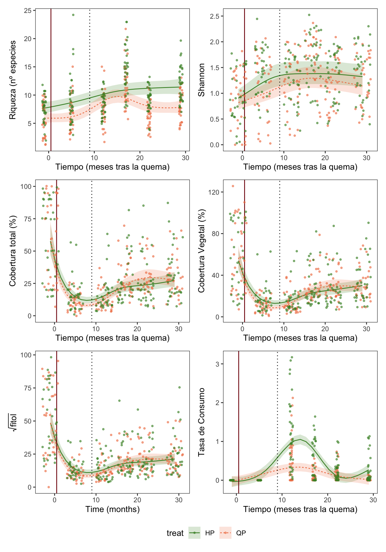
We used Generalizad Additive Mixed Models (GAMM) to evaluate the effects of treatment (Prescribed Fires vs. Pyric herbivorism) on the evolution of plant cover, phytovolumen and diversity indices (Shannon, Richness).
We modelling the date after fire (in months; meses) as smoother (s(meses))
Date after fire and treatment was include as fixed effects
Quadrats were included as random
Different distribution family (e.g. Poisson, Negative Binomial, etc) were used.

Richness

Model

f <- as.formula(riq ~ s(meses, by = treat, k=5, bs="cs") + treat)

m <- gamm(f,
          random = list(quadrat = ~1), 
          data = veg, 
          family = poisson)


 Maximum number of PQL iterations:  20

# Distribution of Model Family

Predicted Distribution of Residuals

      Distribution Probability
            normal         66%
           tweedie         31%
 negative binomial          3%

Predicted Distribution of Response

               Distribution Probability
              beta-binomial         59%
          negative binomial         12%
 neg. binomial (zero-infl.)          9%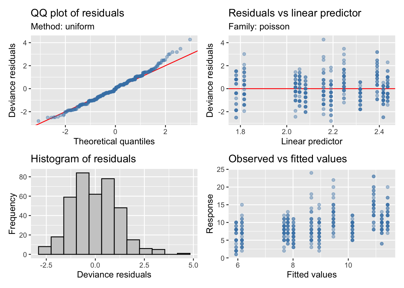

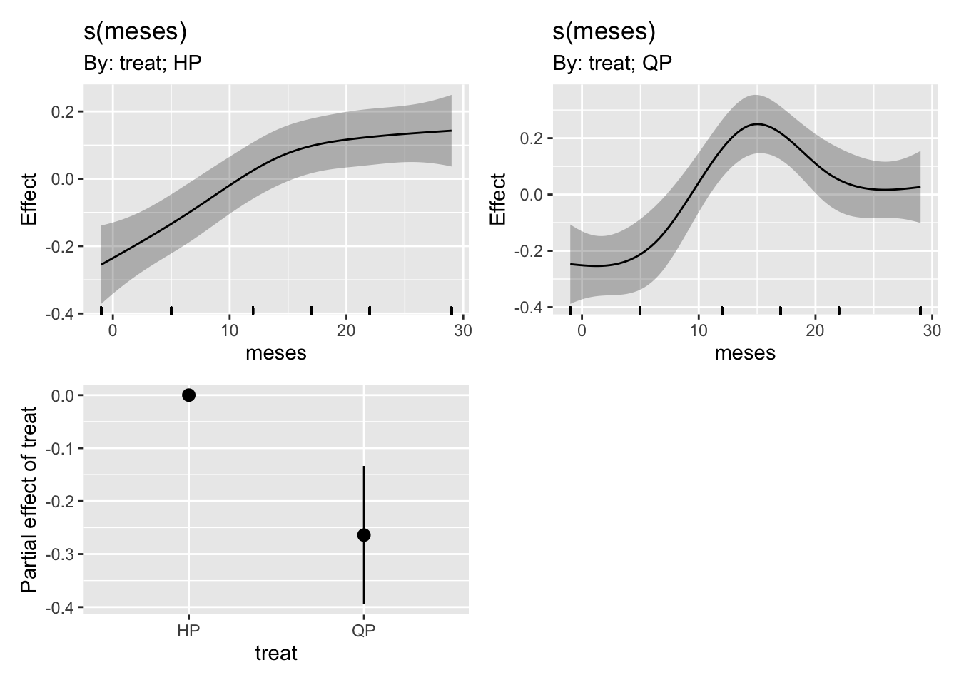
Model validation

Version	Author	Date
5300bc8	ajpelu	2021-10-13

Coefficients

A. parametric coefficients	Estimate	Std. Error	t-value	p-value
(Intercept)	2.2929	0.0462	49.6501	< 0.0001
treatQP	-0.2641	0.0666	-3.9679	0.0001
B. smooth terms	edf	Ref.df	F-value	p-value
s(meses):treatHP	2.2348	4.0000	9.8769	< 0.0001
s(meses):treatQP	3.5900	4.0000	11.6368	< 0.0001

Visualizing effects

Version	Author	Date
5300bc8	ajpelu	2021-10-13

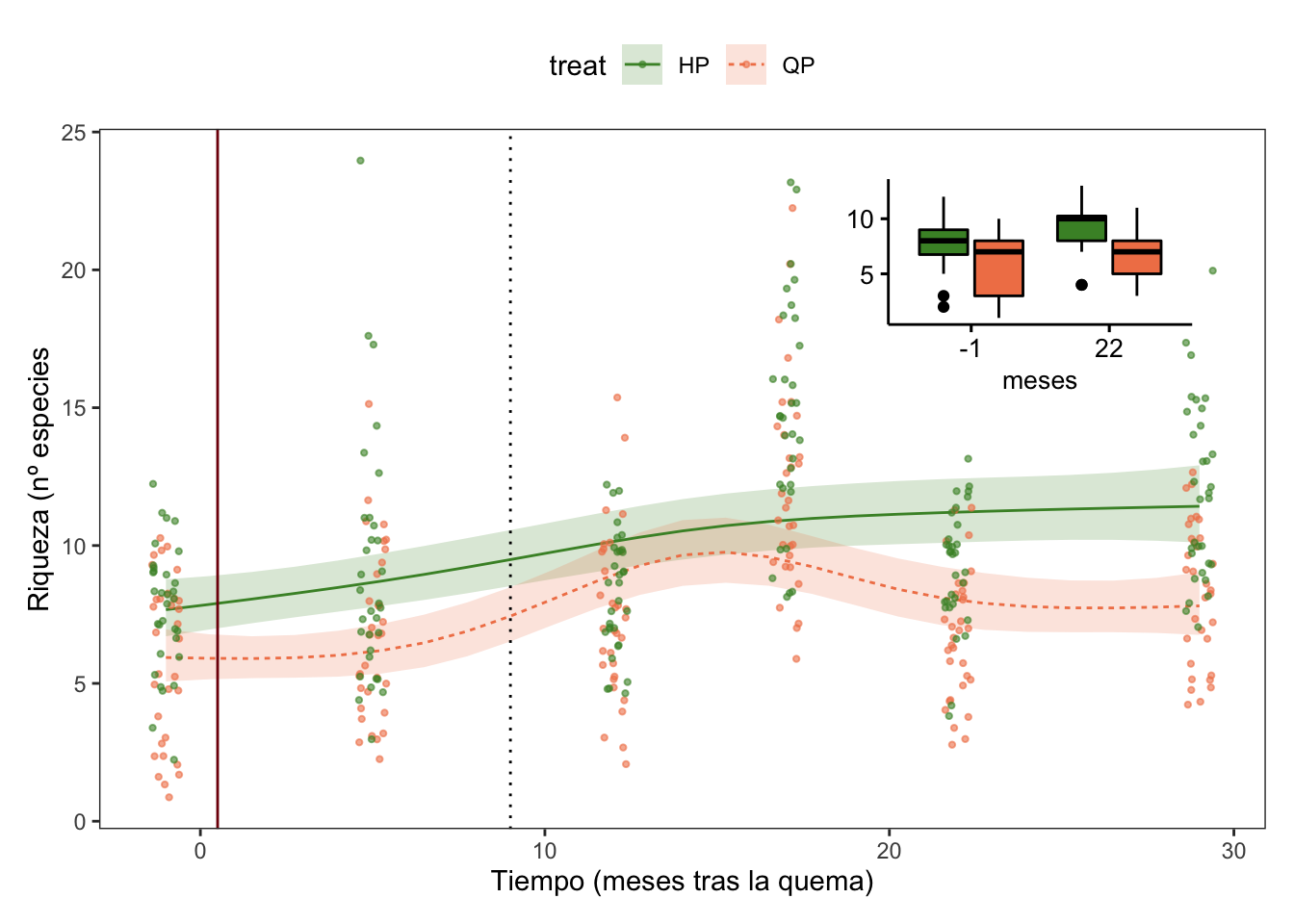
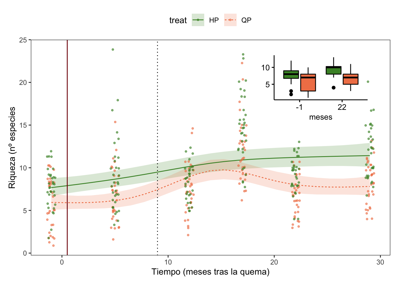
Pre-post (autumn)

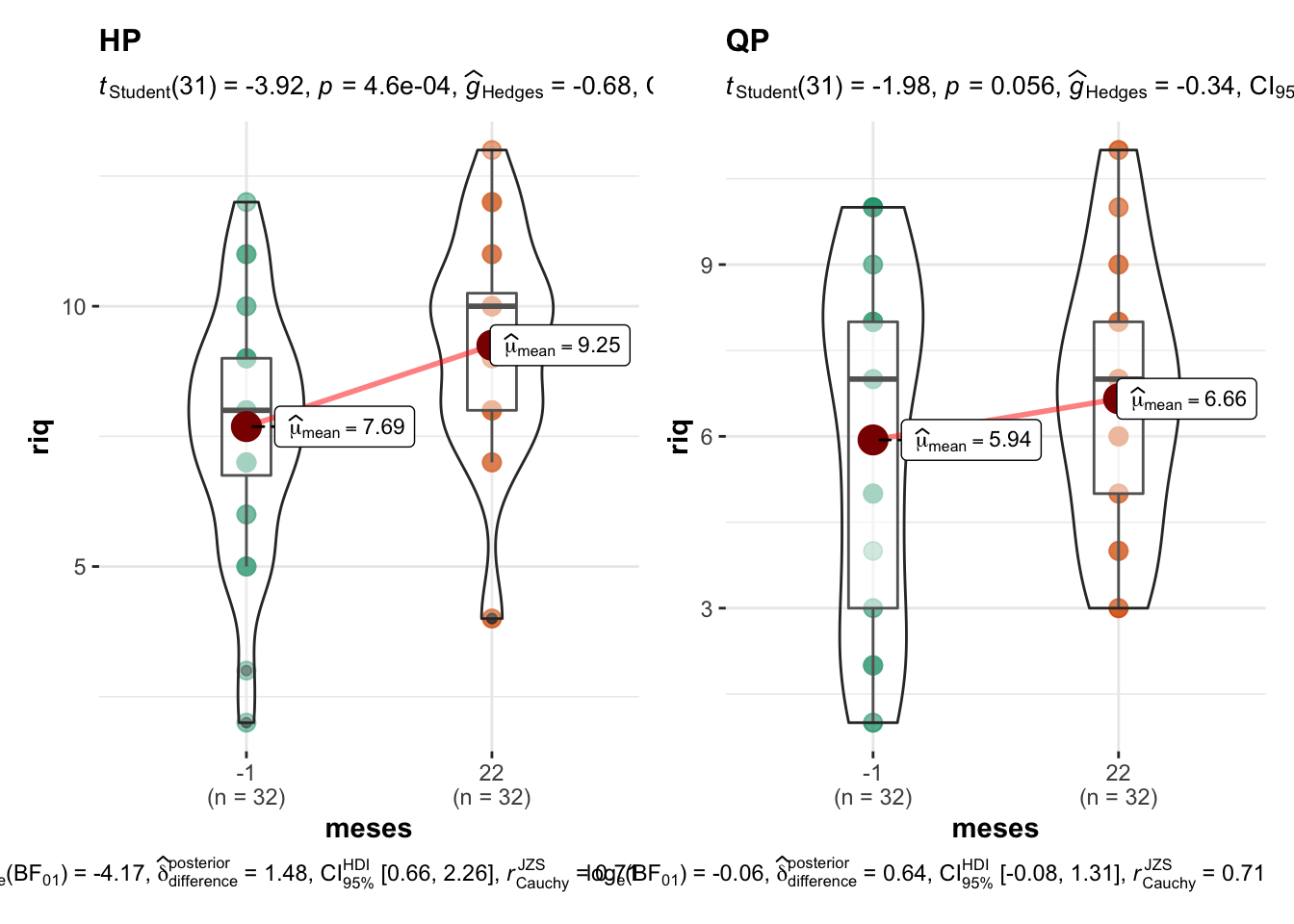
treat	meses	contrast	estimate	SE	df	t.ratio	p.value
HP	.	22 - (-1)	1.5625	0.6115	124	2.5550	0.0465
QP	.	22 - (-1)	0.7188	0.6115	124	1.1753	0.6701
.	-1	QP - HP	-1.7500	0.6115	124	-2.8616	0.0196
.	22	QP - HP	-2.5938	0.6115	124	-4.2414	0.0002

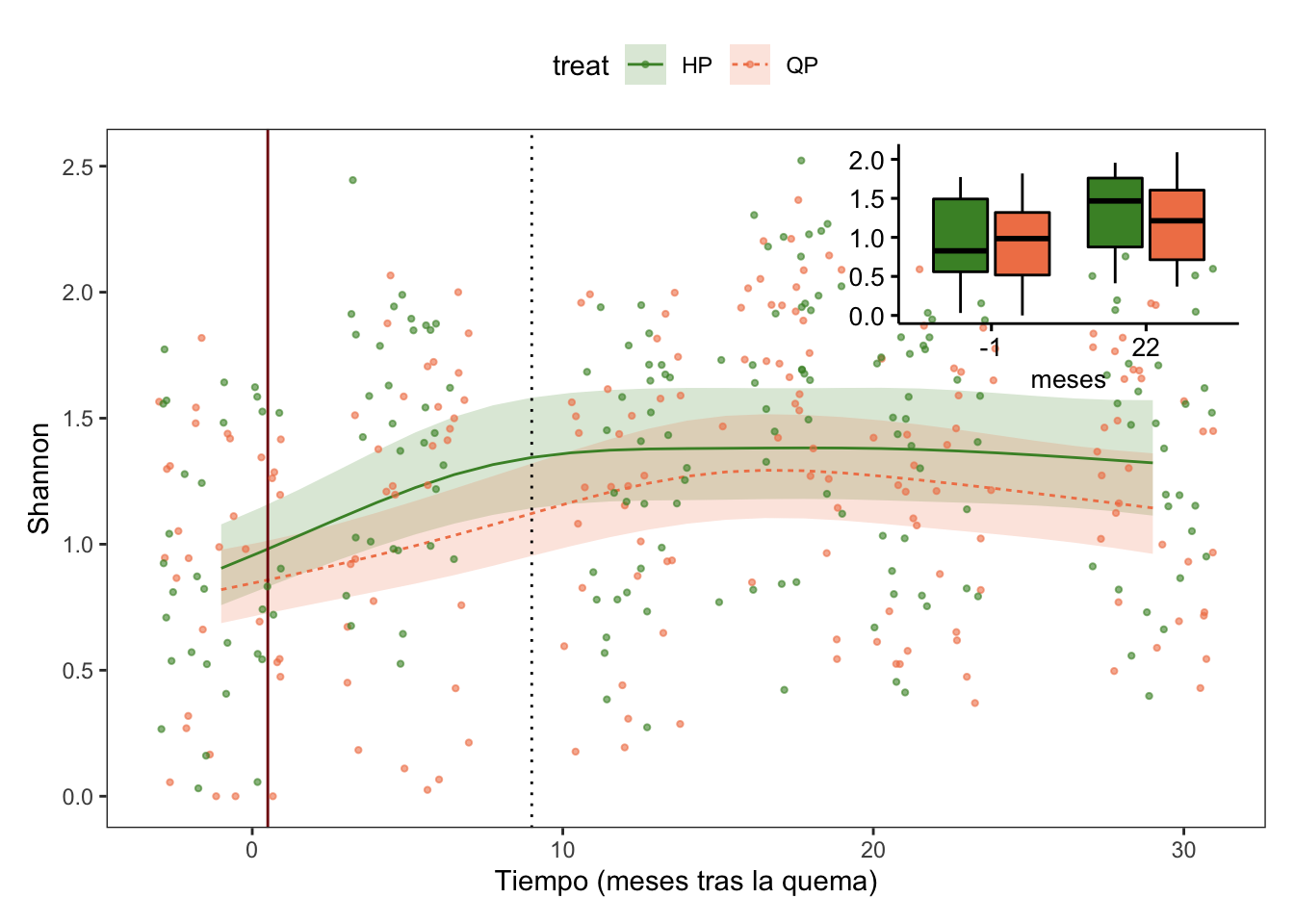
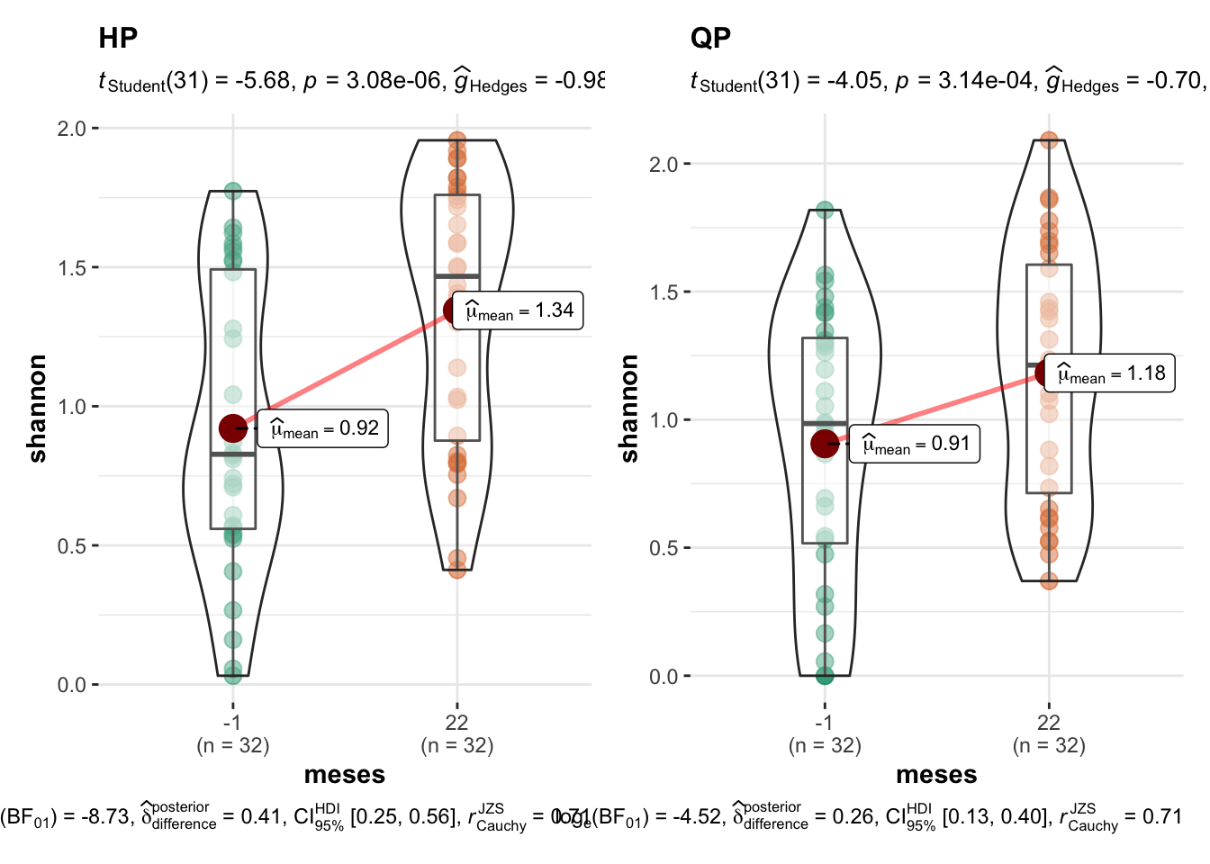
Shannon

Model

veg$shannon <- abs(veg$shan)

f <- as.formula(shannon ~ s(meses, by = treat, k=5, bs="cs") + treat)

m <- gamm(f, 
          random = list(quadrat = ~1), 
          data = veg, 
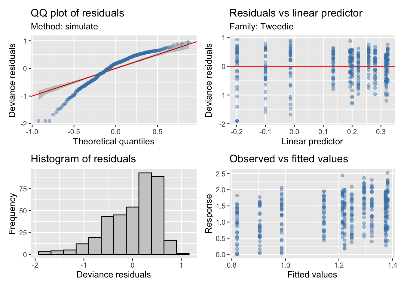
          family = tw)


 Maximum number of PQL iterations:  20

# Distribution of Model Family

Predicted Distribution of Residuals

 Distribution Probability
       normal         50%
         beta         12%
      tweedie         12%

Predicted Distribution of Response

 Distribution Probability
      tweedie         47%
      weibull         25%
         beta         12%

Model validation

Coefficients

A. parametric coefficients	Estimate	Std. Error	t-value	p-value
(Intercept)	0.2221	0.0765	2.9019	0.0039
treatQP	-0.1219	0.1084	-1.1251	0.2613
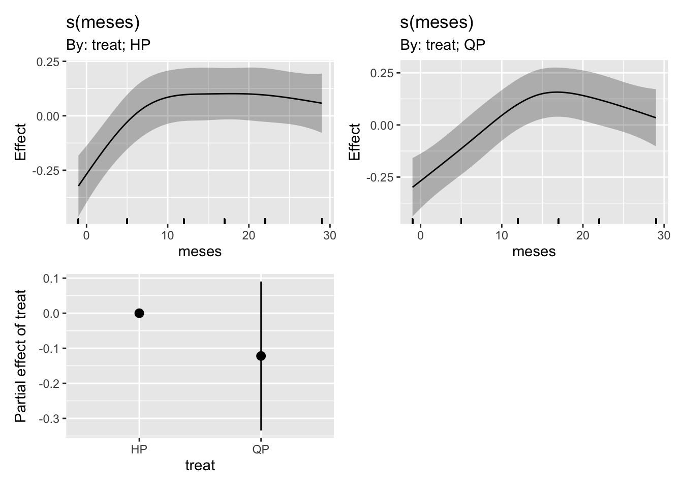
B. smooth terms	edf	Ref.df	F-value	p-value
s(meses):treatHP	2.9693	4.0000	12.7785	< 0.0001
s(meses):treatQP	2.7838	4.0000	14.0029	< 0.0001

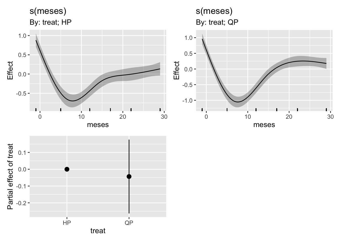
Visualizing effects

Pre-post (autumn)

treat	meses	contrast	estimate	SE	df	t.ratio	p.value
HP	.	22 - (-1)	0.4243	0.1253	124	3.3850	0.0038
QP	.	22 - (-1)	0.2765	0.1253	124	2.2061	0.1119
.	-1	QP - HP	-0.0147	0.1253	124	-0.1170	0.9999
.	22	QP - HP	-0.1624	0.1253	124	-1.2959	0.5851

Total Cover

Model

f <- as.formula(rec_tot ~ s(meses, by = treat, k=5, bs="cs") + treat)

m <- gamm(f, 
          random = list(quadrat = ~1), 
          data = veg, 
          family = nb)


 Maximum number of PQL iterations:  20

# Distribution of Model Family

Predicted Distribution of Residuals

 Distribution Probability
       normal         69%
      tweedie         28%
         beta          3%

Predicted Distribution of Response

               Distribution Probability
 neg. binomial (zero-infl.)         91%
              beta-binomial          9%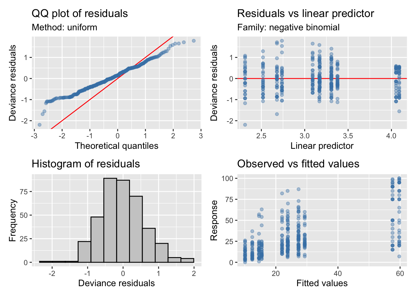

Model validation

Version	Author	Date
5300bc8	ajpelu	2021-10-13

Coefficients

A. parametric coefficients	Estimate	Std. Error	t-value	p-value
(Intercept)	3.1731	0.0793	40.0093	< 0.0001
treatQP	-0.0433	0.1122	-0.3863	0.6995
B. smooth terms	edf	Ref.df	F-value	p-value
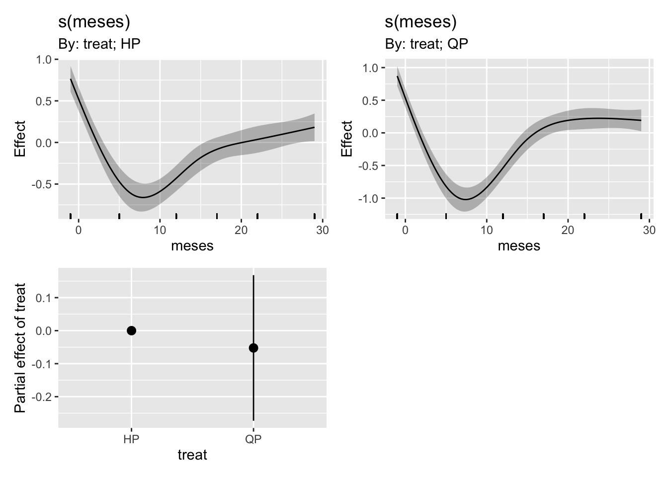
s(meses):treatHP	3.8758	4.0000	53.4401	< 0.0001
s(meses):treatQP	3.9313	4.0000	86.8968	< 0.0001

Visualizing effects

Version	Author	Date
5300bc8	ajpelu	2021-10-13

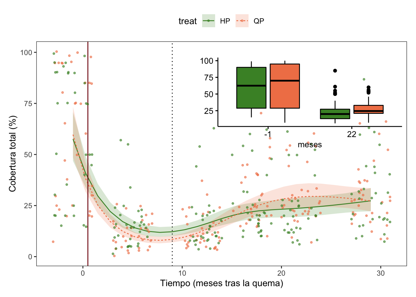
Pre-post (autumn)

treat	meses	contrast	estimate	SE	df	t.ratio	p.value
HP	.	22 - (-1)	-33.2500	6.2205	124	-5.3452	0.0000
QP	.	22 - (-1)	-31.5625	6.2205	124	-5.0739	0.0000
.	-1	QP - HP	1.6563	6.2205	124	0.2663	0.9981
.	22	QP - HP	3.3437	6.2205	124	0.5375	0.9723

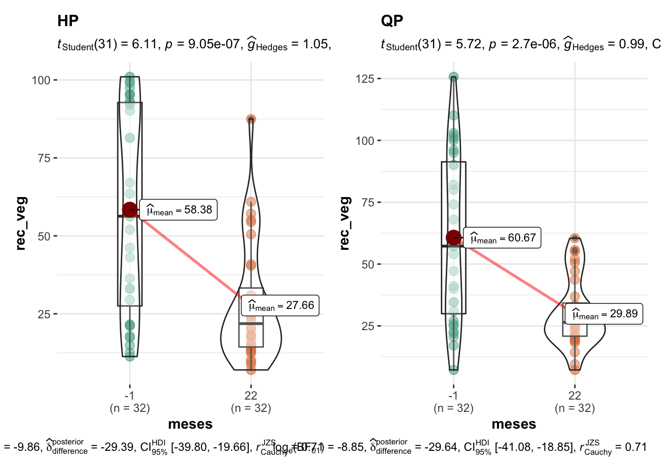
Vegetation Cover

Model

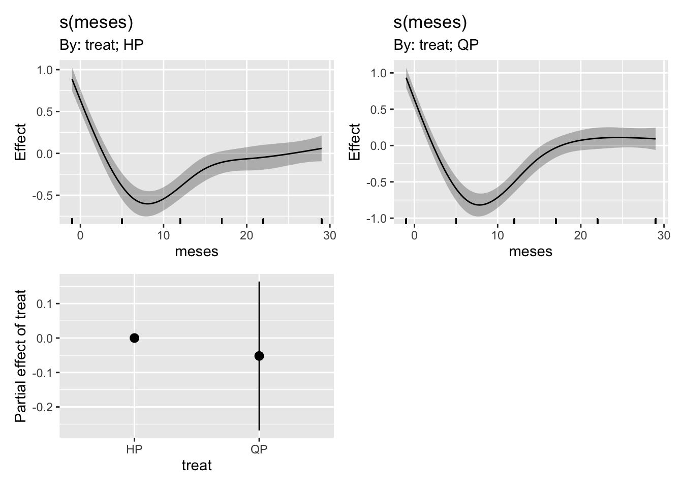
f <- as.formula(rec_veg ~ s(meses, by = treat, k=5, bs="cs") + treat)

m <- gamm(f, 
          random = list(quadrat = ~1), 
          data = veg, 
          family = tw)


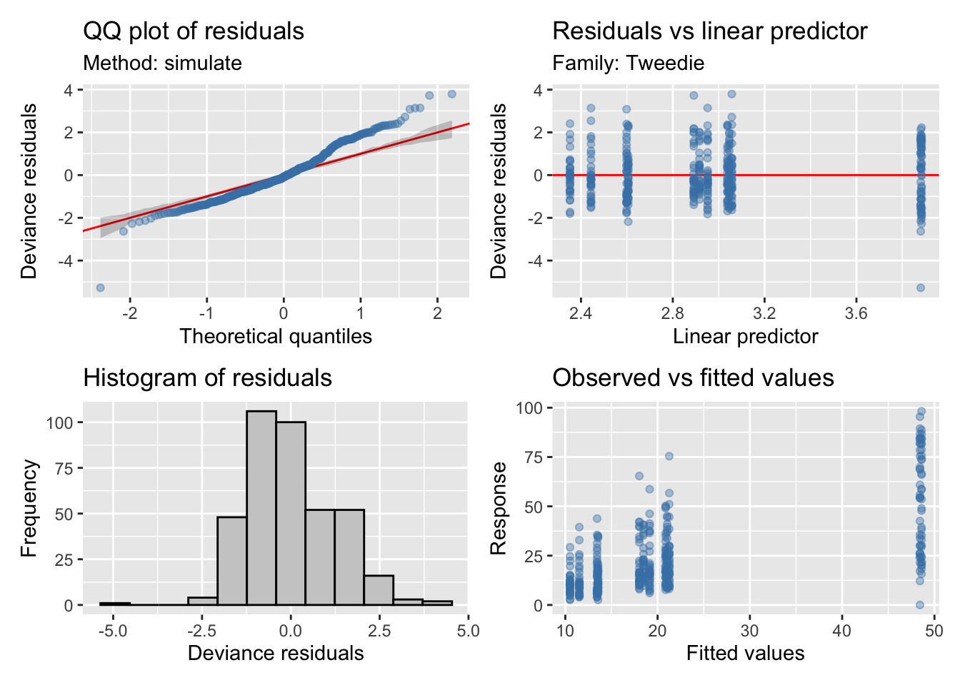
 Maximum number of PQL iterations:  20

# Distribution of Model Family

Predicted Distribution of Residuals

 Distribution Probability
       normal         59%
      tweedie         41%

Predicted Distribution of Response

 Distribution Probability
      tweedie         38%
        gamma         28%
  exponential         12%

Model validation

Version	Author	Date
5300bc8	ajpelu	2021-10-13

Coefficients

A. parametric coefficients	Estimate	Std. Error	t-value	p-value
(Intercept)	3.2225	0.0794	40.5673	< 0.0001
treatQP	-0.0524	0.1125	-0.4656	0.6418
B. smooth terms	edf	Ref.df	F-value	p-value
s(meses):treatHP	3.8507	4.0000	56.3101	< 0.0001
s(meses):treatQP	3.9285	4.0000	82.9721	< 0.0001

Visualizing effects

Pre-post (autumn)

Version	Author	Date
5300bc8	ajpelu	2021-10-13

treat	meses	contrast	estimate	SE	df	t.ratio	p.value
HP	.	22 - (-1)	-30.7187	6.5401	124	-4.6970	0.0000
QP	.	22 - (-1)	-30.7813	6.5401	124	-4.7066	0.0000
.	-1	QP - HP	2.2875	6.5401	124	0.3498	0.9945
.	22	QP - HP	2.2250	6.5401	124	0.3402	0.9950

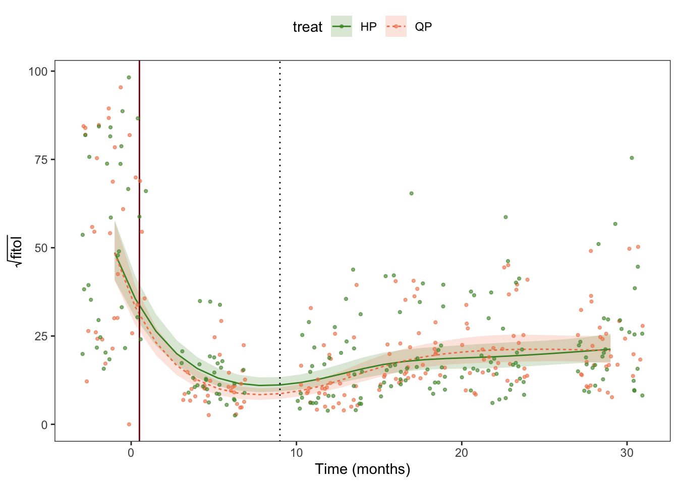
Phytovol

Model

veg$fitovolT <- sqrt(veg$fitovol)
f <- as.formula(fitovolT ~ s(meses, by = treat, k=5, bs="cs") + treat)
m <- gamm(f,
          random = list(quadrat = ~1), 
          data = veg, 
          family = tw)


 Maximum number of PQL iterations:  20

# Distribution of Model Family

Predicted Distribution of Residuals

 Distribution Probability
       normal         69%
      tweedie         31%

Predicted Distribution of Response

               Distribution Probability
                    tweedie         91%
 neg. binomial (zero-infl.)          6%
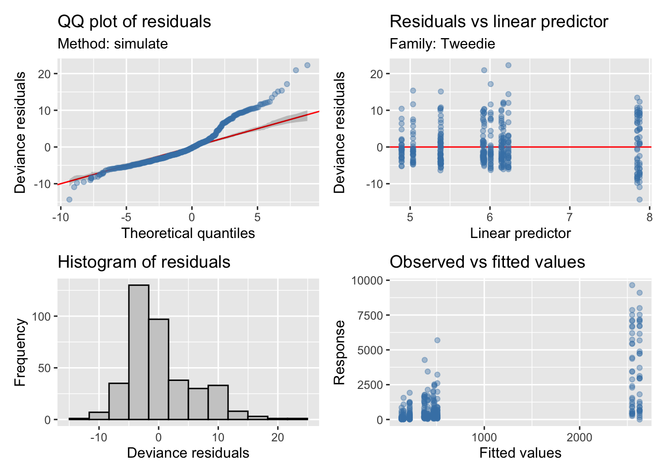
                exponential          3%

Model validation

Coefficients

A. parametric coefficients	Estimate	Std. Error	t-value	p-value
(Intercept)	2.9981	0.0779	38.4854	< 0.0001
treatQP	-0.0521	0.1103	-0.4721	0.6371
B. smooth terms	edf	Ref.df	F-value	p-value
s(meses):treatHP	3.8902	4.0000	94.7206	< 0.0001
s(meses):treatQP	3.9261	4.0000	113.2126	< 0.0001

Visualizing effects

Version	Author	Date
5300bc8	ajpelu	2021-10-13

Phytovol (I)

Model

f <- as.formula(fitovol ~ s(meses, by = treat, k=5, bs="cs") + treat)
m <- gamm(f,
          random = list(quadrat = ~1), 
          data = veg, 
          family = tw)


 Maximum number of PQL iterations:  20

# Distribution of Model Family

Predicted Distribution of Residuals

 Distribution Probability
       normal         50%
      tweedie         50%

Predicted Distribution of Response

 Distribution Probability
    lognormal         31%
      tweedie         22%
            F         16%

Model validation

Coefficients

A. parametric coefficients	Estimate	Std. Error	t-value	p-value
(Intercept)	6.1291	0.1537	39.8752	< 0.0001
treatQP	-0.1246	0.2179	-0.5720	0.5676
B. smooth terms	edf	Ref.df	F-value	p-value
s(meses):treatHP	3.8933	4.0000	129.0408	< 0.0001
s(meses):treatQP	3.9218	4.0000	148.4011	< 0.0001

Visualizing effects

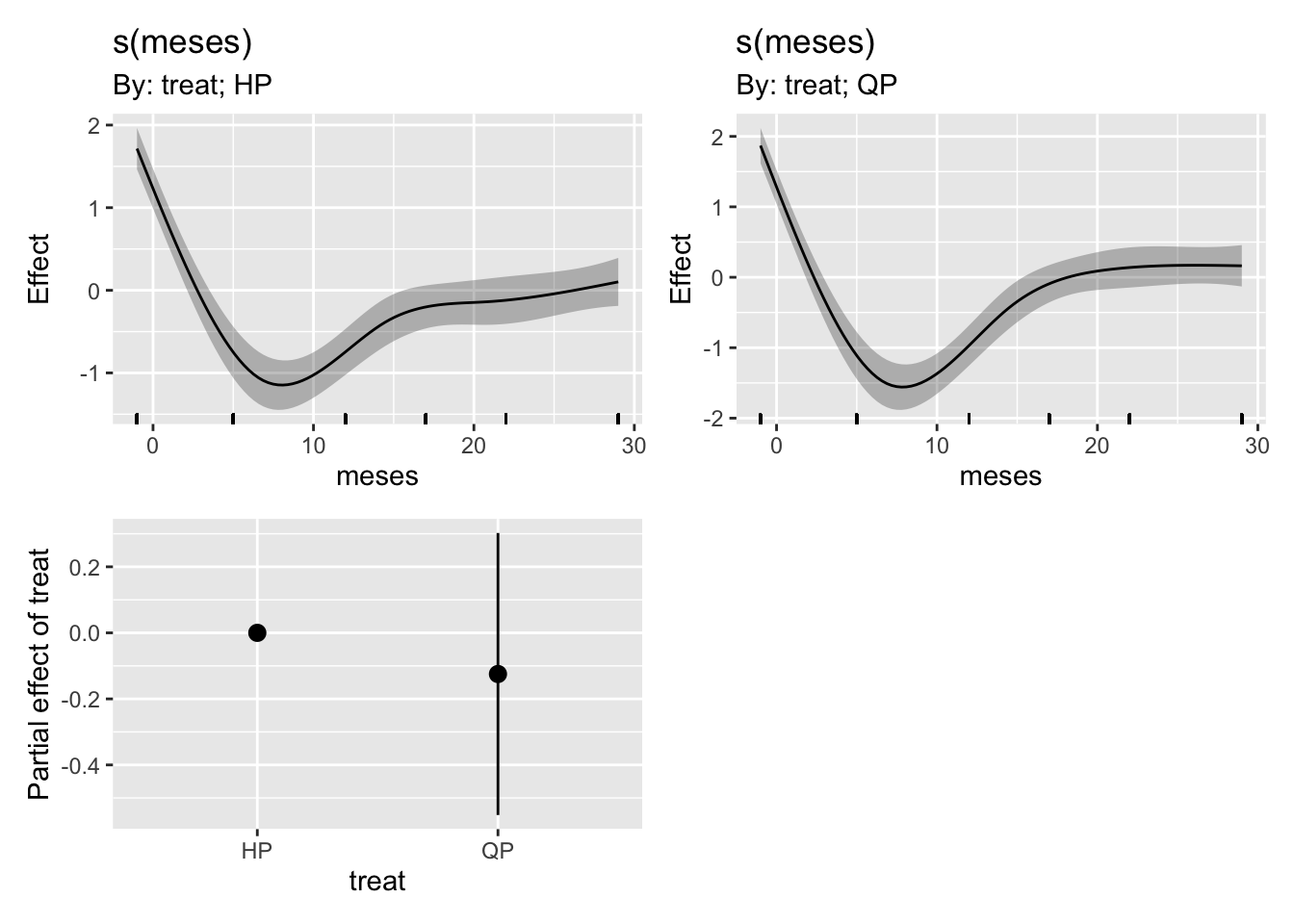
Pre-post (autumn)

Version	Author	Date
bbd9ef6	ajpelu	2021-10-13

treat	meses	contrast	estimate	SE	df	t.ratio	p.value
HP	.	22 - (-1)	-2802.6813	519.4577	124	-5.3954	0.0000
QP	.	22 - (-1)	-2865.2197	519.4577	124	-5.5158	0.0000
.	-1	QP - HP	67.2869	519.4577	124	0.1295	0.9999
.	22	QP - HP	4.7484	519.4577	124	0.0091	1.0000

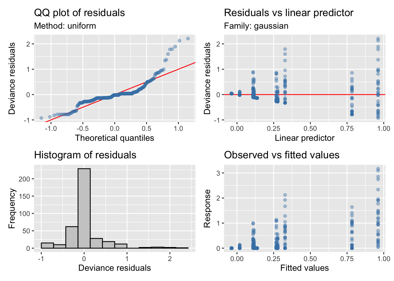
Tasa consumo

Model

Caution, there is an outlier .

veg %>% filter(consumo > 8)

# A tibble: 1 x 15
  zona    parcela quadrat rango_infoca fecha               rec_tot rec_veg   riq
  <chr>   <chr>   <fct>          <dbl> <dttm>                <dbl>   <dbl> <dbl>
1 Quemad… AL_P_14 P14Q8              4 2020-05-19 00:00:00      16      20    17
# … with 7 more variables: shan <dbl>, fitovol <dbl>, consumo <dbl>,
#   treat <fct>, meses <dbl>, shannon <dbl>, fitovolT <dbl>

f <- as.formula(consumo ~ s(meses, by = treat, k=5, bs="cs") + treat)

veg.out <- veg %>% filter(consumo < 8)
ad.out <- ad %>% filter(consumo < 8)

m <- gamm(f, 
          random = list(quadrat = ~1), 
          data = veg.out)

# Distribution of Model Family

Predicted Distribution of Residuals

 Distribution Probability
       normal         53%
      tweedie         31%
         beta         12%

Predicted Distribution of Response

         Distribution Probability
              tweedie         88%
                 beta          6%
 poisson (zero-infl.)          6%

Model validation

Coefficients

A. parametric coefficients	Estimate	Std. Error	t-value	p-value
(Intercept)	0.3678	0.0362	10.1564	< 0.0001
treatQP	-0.2283	0.0512	-4.4610	< 0.0001
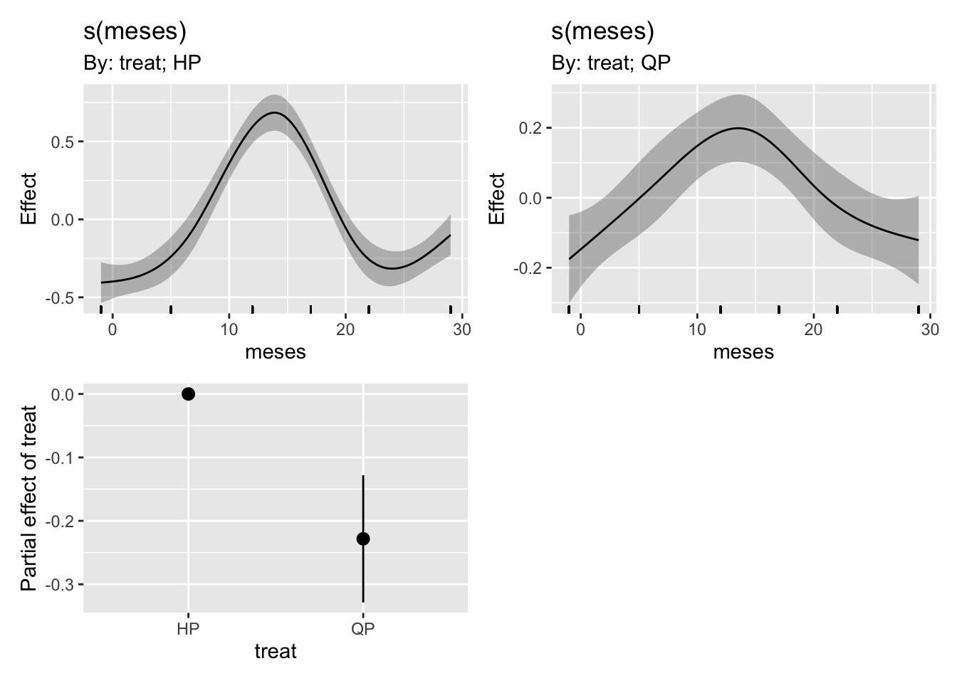
B. smooth terms	edf	Ref.df	F-value	p-value
s(meses):treatHP	3.9324	4.0000	45.6797	< 0.0001
s(meses):treatQP	3.0710	4.0000	6.2542	< 0.0001

Visualizing effects

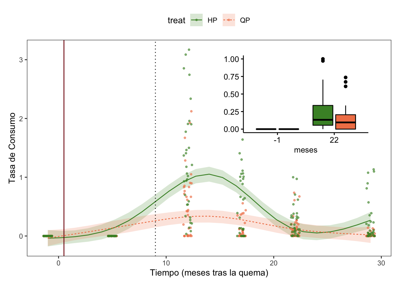
Pre-post (autumn)

treat	meses	contrast	estimate	SE	df	t.ratio	p.value
HP	.	22 - (-1)	0.2454	0.0417	124	5.8793	0.0000
QP	.	22 - (-1)	0.1503	0.0417	124	3.6021	0.0018
.	-1	QP - HP	0.0000	0.0417	124	0.0000	1.0000
.	22	QP - HP	-0.0950	0.0417	124	-2.2771	0.0944

General overview

Parametric terms

Variable	term	Estimate	SE	F	p
Richness	treatHP	2.293	0.046	49.65	< 0.0001
Richness	treatQP	-0.264	0.067	-3.97	< 0.0001
Shannon	treatHP	0.222	0.077	2.90	0.0039
Shannon	treatQP	-0.122	0.108	-1.13	0.2613
Total cover	treatHP	3.173	0.079	40.01	< 0.0001
Total cover	treatQP	-0.043	0.112	-0.39	0.6995
Veg. cover	treatHP	3.222	0.079	40.57	< 0.0001
Veg. cover	treatQP	-0.052	0.113	-0.47	0.6418
Fitovol	treatHP	2.998	0.078	38.49	< 0.0001
Fitovol	treatQP	-0.052	0.110	-0.47	0.6371
Fitovol	treatHP	6.129	0.154	39.88	< 0.0001
Fitovol	treatQP	-0.125	0.218	-0.57	0.5676
Tasa Consumo	treatHP	0.368	0.036	10.16	< 0.0001
Tasa Consumo	treatQP	-0.228	0.051	-4.46	< 0.0001

Smooth terms

Variable	term	edf	ref.df	F	p
Richness	s(meses):treatHP	2.235	4	9.88	< 0.0001
Richness	s(meses):treatQP	3.590	4	11.64	< 0.0001
Shannon	s(meses):treatHP	2.969	4	12.78	< 0.0001
Shannon	s(meses):treatQP	2.784	4	14.00	< 0.0001
Total cover	s(meses):treatHP	3.876	4	53.44	< 0.0001
Total cover	s(meses):treatQP	3.931	4	86.90	< 0.0001
Veg. cover	s(meses):treatHP	3.851	4	56.31	< 0.0001
Veg. cover	s(meses):treatQP	3.929	4	82.97	< 0.0001
Fitovol	s(meses):treatHP	3.890	4	94.72	< 0.0001
Fitovol	s(meses):treatQP	3.926	4	113.21	< 0.0001
Fitovol	s(meses):treatHP	3.893	4	129.04	< 0.0001
Fitovol	s(meses):treatQP	3.922	4	148.40	< 0.0001
Tasa Consumo	s(meses):treatHP	3.932	4	45.68	< 0.0001
Tasa Consumo	s(meses):treatQP	3.071	4	6.25	< 0.0001

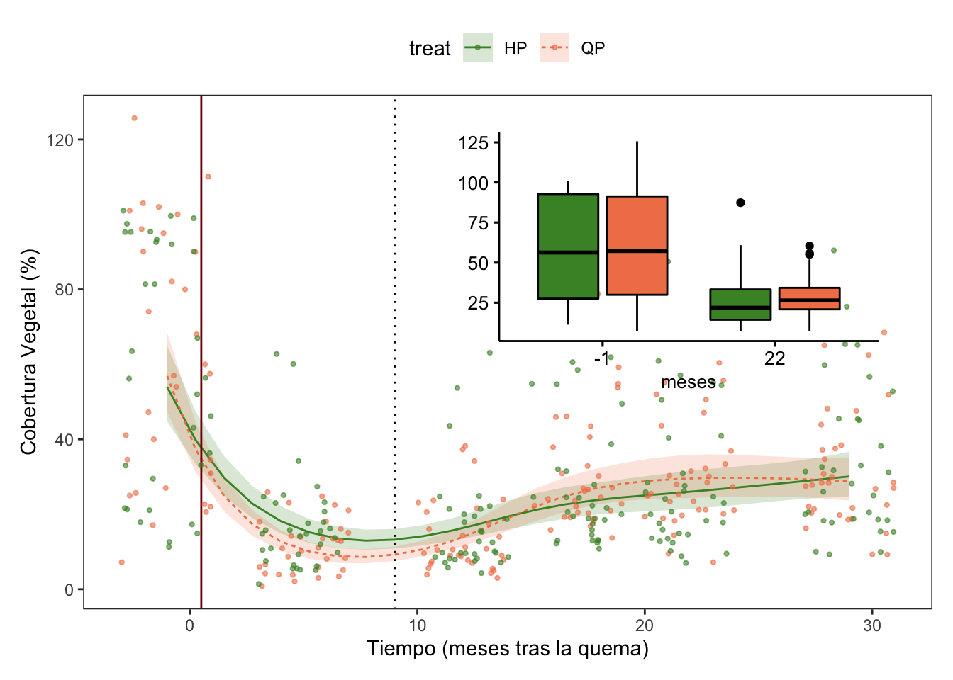
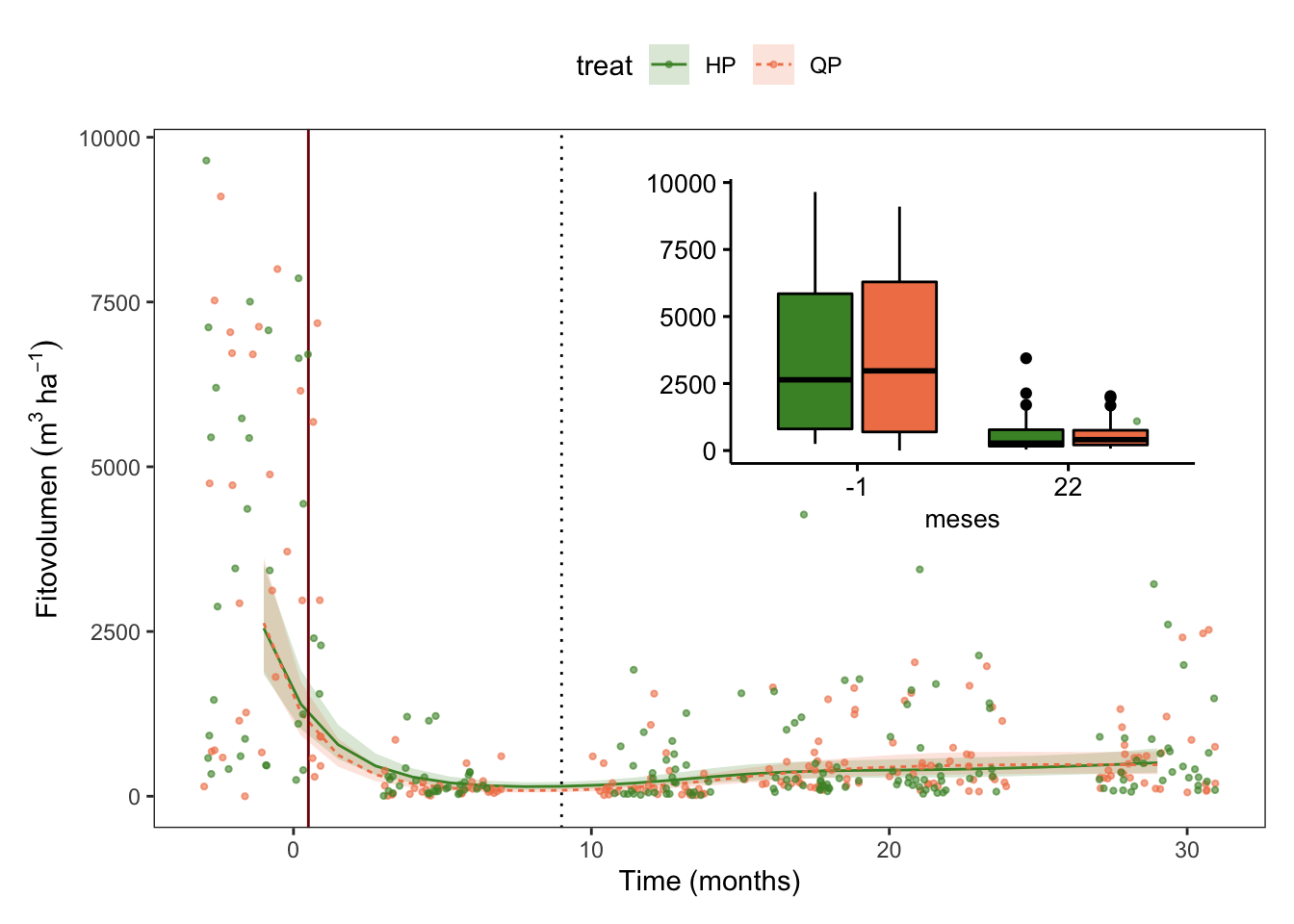
All plots

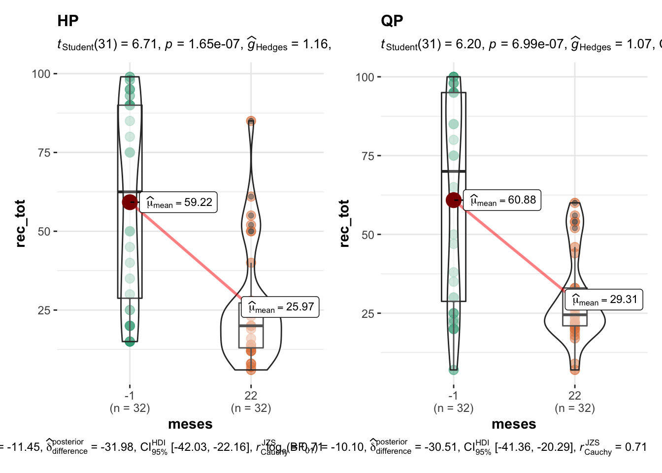
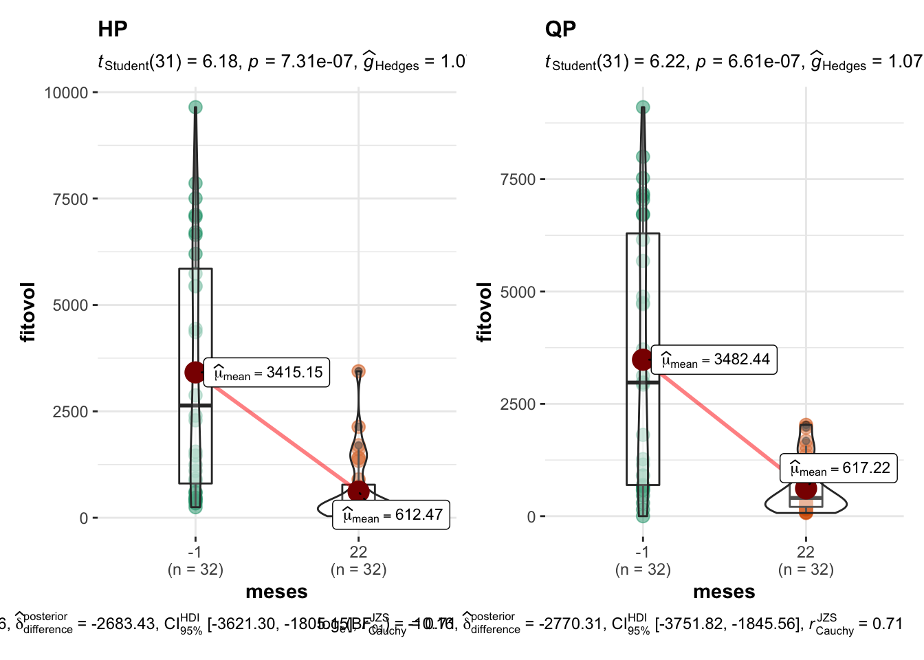
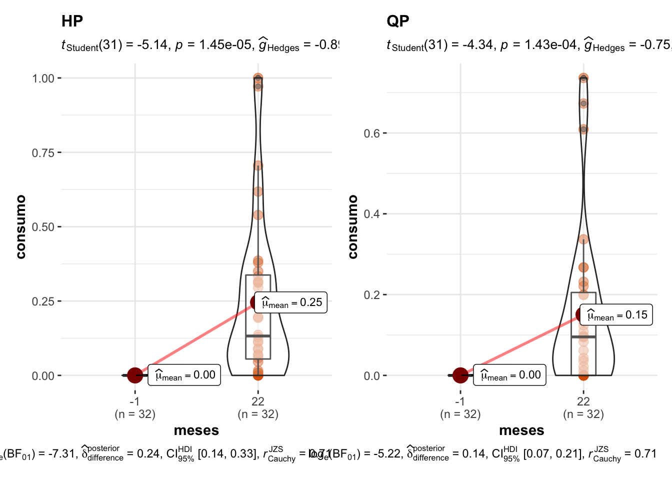
Comparison before-after

Summary table

Characteristic	HP		QP
Characteristic	-1, N = 32¹	22, N = 32¹	-1, N = 32¹	22, N = 32¹
rec_tot	59.22 ± 5.42	25.97 ± 3.25	60.88 ± 5.61	29.31 ± 2.44
rec_veg	58.38 ± 5.78	27.66 ± 3.34	60.67 ± 5.92	29.89 ± 2.42
riq	7.69 ± 0.41	9.25 ± 0.38	5.94 ± 0.53	6.66 ± 0.41
shan	-0.92 ± 0.09	-1.34 ± 0.08	-0.91 ± 0.09	-1.18 ± 0.09
fitovol	3,415.15 ± 502.49	612.47 ± 135.99	3,482.44 ± 508.21	617.22 ± 101.99
consumo	0.00 ± 0.00	0.25 ± 0.05	0.00 ± 0.00	0.15 ± 0.03
¹ Mean ± std.error

Some resources

Plots for Generalized Additive Models
Family distributions for GAMs
Tidy Model Visualisation for Generalised Additive Models
Course about GAMs
Hierarchical generalized additive models in ecology: an introduction with mgcv paper
GAMs

R version 4.0.2 (2020-06-22)
Platform: x86_64-apple-darwin17.0 (64-bit)
Running under: macOS Catalina 10.15.3

Matrix products: default
BLAS:   /Library/Frameworks/R.framework/Versions/4.0/Resources/lib/libRblas.dylib
LAPACK: /Library/Frameworks/R.framework/Versions/4.0/Resources/lib/libRlapack.dylib

locale:
[1] en_US.UTF-8/en_US.UTF-8/en_US.UTF-8/C/en_US.UTF-8/en_US.UTF-8

attached base packages:
[1] stats     graphics  grDevices utils     datasets  methods   base     

other attached packages:
 [1] plotrix_3.8-1     gtsummary_1.4.2   emmeans_1.5.4     patchwork_1.1.1  
 [5] performance_0.7.2 broom_0.7.9       tidymv_3.2.1      kableExtra_1.3.1 
 [9] itsadug_2.4       plotfunctions_1.4 gratia_0.6.0      mgcv_1.8-33      
[13] nlme_3.1-152      janitor_2.1.0     here_1.0.1        forcats_0.5.1    
[17] stringr_1.4.0     dplyr_1.0.6       purrr_0.3.4       readr_1.4.0      
[21] tidyr_1.1.3       tibble_3.1.2      ggplot2_3.3.5     tidyverse_1.3.1  
[25] workflowr_1.6.2  

loaded via a namespace (and not attached):
  [1] readxl_1.3.1              pairwiseComparisons_3.1.3
  [3] backports_1.2.1           plyr_1.8.6               
  [5] splines_4.0.2             gmp_0.6-2                
  [7] kSamples_1.2-9            ipmisc_5.0.2             
  [9] TH.data_1.0-10            digest_0.6.27            
 [11] SuppDists_1.1-9.5         htmltools_0.5.2          
 [13] fansi_0.4.2               checkmate_2.0.0          
 [15] magrittr_2.0.1            memoise_2.0.0            
 [17] paletteer_1.3.0           openxlsx_4.2.3           
 [19] modelr_0.1.8              sandwich_3.0-0           
 [21] colorspace_2.0-0          rvest_1.0.0              
 [23] ggrepel_0.9.1             haven_2.3.1              
 [25] xfun_0.23                 prismatic_1.0.0          
 [27] crayon_1.4.1              jsonlite_1.7.2           
 [29] zeallot_0.1.0             survival_3.2-7           
 [31] zoo_1.8-8                 glue_1.4.2               
 [33] gtable_0.3.0              webshot_0.5.2            
 [35] MatrixModels_0.4-1        statsExpressions_1.1.0   
 [37] car_3.0-10                Rmpfr_0.8-2              
 [39] abind_1.4-5               scales_1.1.1             
 [41] mvtnorm_1.1-1             DBI_1.1.1                
 [43] rstatix_0.6.0             PMCMRplus_1.9.0          
 [45] Rcpp_1.0.7                viridisLite_0.3.0        
 [47] xtable_1.8-4              foreign_0.8-81           
 [49] tweedie_2.3.3             httr_1.4.2               
 [51] RColorBrewer_1.1-2        ellipsis_0.3.2           
 [53] reshape_0.8.8             pkgconfig_2.0.3          
 [55] farver_2.0.3              multcompView_0.1-8       
 [57] sass_0.3.1                dbplyr_2.1.1             
 [59] utf8_1.1.4                effectsize_0.4.5         
 [61] tidyselect_1.1.1          labeling_0.4.2           
 [63] rlang_0.4.10              later_1.1.0.1            
 [65] ggcorrplot_0.1.3          munsell_0.5.0            
 [67] cellranger_1.1.0          tools_4.0.2              
 [69] cachem_1.0.4              cli_2.5.0                
 [71] generics_0.1.0            evaluate_0.14            
 [73] fastmap_1.1.0             BWStest_0.2.2            
 [75] yaml_2.2.1                rematch2_2.1.2           
 [77] knitr_1.31                fs_1.5.0                 
 [79] zip_2.1.1                 randomForest_4.6-14      
 [81] WRS2_1.1-1                pbapply_1.4-3            
 [83] whisker_0.4               mvnfast_0.2.7            
 [85] xml2_1.3.2                correlation_0.6.1        
 [87] compiler_4.0.2            rstudioapi_0.13          
 [89] curl_4.3                  ggsignif_0.6.0           
 [91] gt_0.3.0                  reprex_2.0.0             
 [93] broom.helpers_1.4.0       bslib_0.2.4              
 [95] stringi_1.7.4             parameters_0.14.0        
 [97] highr_0.8                 lattice_0.20-41          
 [99] Matrix_1.3-2              commonmark_1.7           
[101] vctrs_0.3.8               mc2d_0.1-18              
[103] pillar_1.6.1              lifecycle_1.0.0          
[105] jquerylib_0.1.3           estimability_1.3         
[107] data.table_1.14.0         insight_0.14.4           
[109] httpuv_1.5.5              R6_2.5.0                 
[111] promises_1.2.0.1          rio_0.5.16               
[113] BayesFactor_0.9.12-4.2    codetools_0.2-18         
[115] MASS_7.3-53               gtools_3.8.2             
[117] assertthat_0.2.1          rprojroot_2.0.2          
[119] withr_2.4.1               multcomp_1.4-16          
[121] bayestestR_0.9.0          parallel_4.0.2           
[123] hms_1.0.0                 grid_4.0.2               
[125] coda_0.19-4               rmarkdown_2.8            
[127] snakecase_0.11.0          carData_3.0-4            
[129] git2r_0.28.0              ggpubr_0.4.0             
[131] lubridate_1.7.10          ggstatsplot_0.7.2

temporal_analysis

ajpelu

2021-10-07

Introduction

Statistical analysis

Richness

Model

Model validation

Coefficients

Visualizing effects

Pre-post (autumn)

Shannon

Model

Model validation

Coefficients

Visualizing effects

Pre-post (autumn)

Total Cover

Model

Model validation

Coefficients

Visualizing effects

Pre-post (autumn)

Vegetation Cover

Model

Model validation

Coefficients

Visualizing effects

Pre-post (autumn)

Phytovol

Model

Model validation

Coefficients

Visualizing effects

Phytovol (I)

Model

Model validation

Coefficients

Visualizing effects

Pre-post (autumn)

Tasa consumo

Model

Model validation

Coefficients

Visualizing effects

Pre-post (autumn)

General overview

All plots

Comparison before-after

Summary table

Some resources