compara_methods
ajpelu
2022-02-02
Last updated: 2022-04-13
Checks: 7 0
Knit directory: veg_alcontar/
This reproducible R Markdown analysis was created with workflowr (version 1.7.0). The Checks tab describes the reproducibility checks that were applied when the results were created. The Past versions tab lists the development history.
Great! Since the R Markdown file has been committed to the Git repository, you know the exact version of the code that produced these results.
Great job! The global environment was empty. Objects defined in the global environment can affect the analysis in your R Markdown file in unknown ways. For reproduciblity it’s best to always run the code in an empty environment.
The command set.seed(20211007) was run prior to running the code in the R Markdown file. Setting a seed ensures that any results that rely on randomness, e.g. subsampling or permutations, are reproducible.
Great job! Recording the operating system, R version, and package versions is critical for reproducibility.
Nice! There were no cached chunks for this analysis, so you can be confident that you successfully produced the results during this run.
Great job! Using relative paths to the files within your workflowr project makes it easier to run your code on other machines.
Great! You are using Git for version control. Tracking code development and connecting the code version to the results is critical for reproducibility.
The results in this page were generated with repository version 1d91b1b. See the Past versions tab to see a history of the changes made to the R Markdown and HTML files.
Note that you need to be careful to ensure that all relevant files for the analysis have been committed to Git prior to generating the results (you can use wflow_publish or wflow_git_commit). workflowr only checks the R Markdown file, but you know if there are other scripts or data files that it depends on. Below is the status of the Git repository when the results were generated:
Ignored files:
    Ignored:    .Rhistory
    Ignored:    .Rproj.user/

Untracked files:
    Untracked:  data/Cobertura_fitovolumen_corregido_parcela.xlsx

Unstaged changes:
    Modified:   output/paper_SUDOE/compara_cobertura.jpg
Note that any generated files, e.g. HTML, png, CSS, etc., are not included in this status report because it is ok for generated content to have uncommitted changes.
These are the previous versions of the repository in which changes were made to the R Markdown (analysis/compara_methods.Rmd) and HTML (docs/compara_methods.html) files. If you’ve configured a remote Git repository (see ?wflow_git_remote), click on the hyperlinks in the table below to view the files as they were in that past version.
| File | Version | Author | Date | Message |
|---|---|---|---|---|
| Rmd | 1d91b1b | ajpelu | 2022-04-13 | add correlation qp-qmp |
| html | 5a89fea | ajpelu | 2022-04-13 | Build site. |
| Rmd | 8ac0cd2 | ajpelu | 2022-04-13 | add new analysis |
| html | a3d3eb4 | ajpelu | 2022-04-01 | Build site. |
| Rmd | 2a0a2cb | ajpelu | 2022-04-01 | update analysis paper sudoe |
| html | b4ebf2e | ajpelu | 2022-04-01 | Build site. |
| Rmd | a6c71fa | ajpelu | 2022-04-01 | add analysis_SUDOE cobertura |
| Rmd | 1cf2118 | ajpelu | 2022-02-04 | update |
| html | 792adb1 | ajpelu | 2022-02-02 | Build site. |
| Rmd | 179f390 | ajpelu | 2022-02-02 | genera plots compara metodos |
Introduction
Comparison of estimation methods for coverage, phytovolume, richness and diversity (shannon)
- Prepara data
Cobertura
- Summary values
| metodo | mean | sd | se | cv | median | n |
|---|---|---|---|---|---|---|
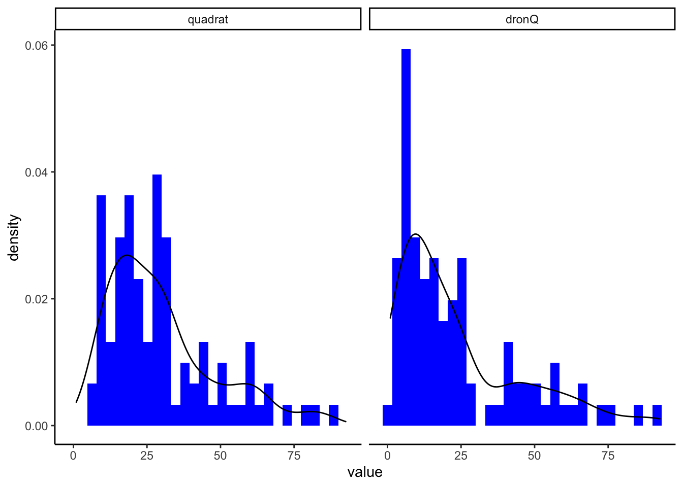
| quadrat | 29.92 | 18.47 | 1.89 | 61.75 | 26.50 | 96 |
| dronQ | 23.55 | 21.01 | 2.14 | 89.23 | 15.74 | 96 |
| line_intercept | 27.19 | 6.49 | 1.87 | 23.86 | 29.67 | 12 |
| point_quadrat | 55.50 | 7.62 | 2.20 | 13.73 | 56.00 | 12 |
| dronT | 17.46 | 2.71 | 0.78 | 15.51 | 17.07 | 12 |
1.1 Comparación cobertura Quadrat - DronQ
Comprobamos Normalidad y Homocedascticidad
Normality?
| Version | Author | Date |
|---|---|---|
| 5a89fea | ajpelu | 2022-04-13 |
    Shapiro-Wilk normality test

data:  cob_selected$value
W = 0.89104, p-value = 1.299e-10
Los resultados indican que los datos no son normales (W = 0.89; p<0.0001)
- Homogeneidad de la varianza?
    Bartlett test of homogeneity of variances

data:  cob_selected$value and cob_selected$metodo
Bartlett's K-squared = 1.5582, df = 1, p-value = 0.2119
Según los resultados, no parece existir heterogeneidad en las varianzas (Bartlett’s K-squared = 1.56; p=0.2119)
Por tanto, dos opciones: aplicar método wilcox.test o transformar datos (log) y aplicar t-test
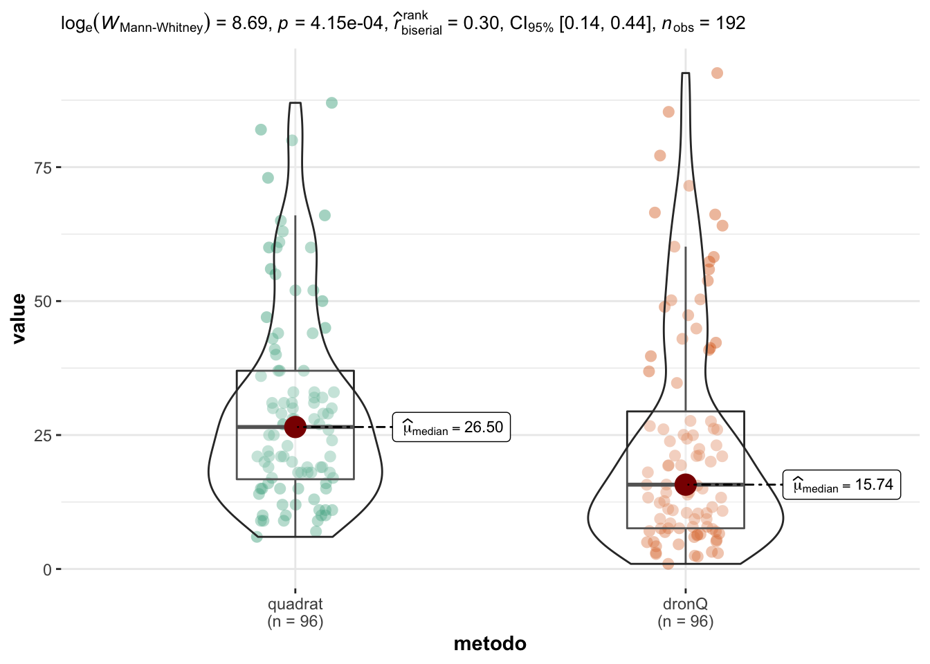
- Wilcox test
    Wilcoxon rank sum test with continuity correction

data:  value by metodo
W = 5967.5, p-value = 0.0004154
alternative hypothesis: true location shift is not equal to 0- T-test de datos transformados (log)
En cualquier caso obtenemos los siguientes resultados: - Existen diferencias significativas tanto si usamos el test no paramétrico de Wilcoxon (W = 5967.5; p=0.0004), como si aplicamos el test paramétrico a los datos transformados (t = 3.997; p<0.0001). De forma gráfica
| Version | Author | Date |
|---|---|---|
| 5a89fea | ajpelu | 2022-04-13 |
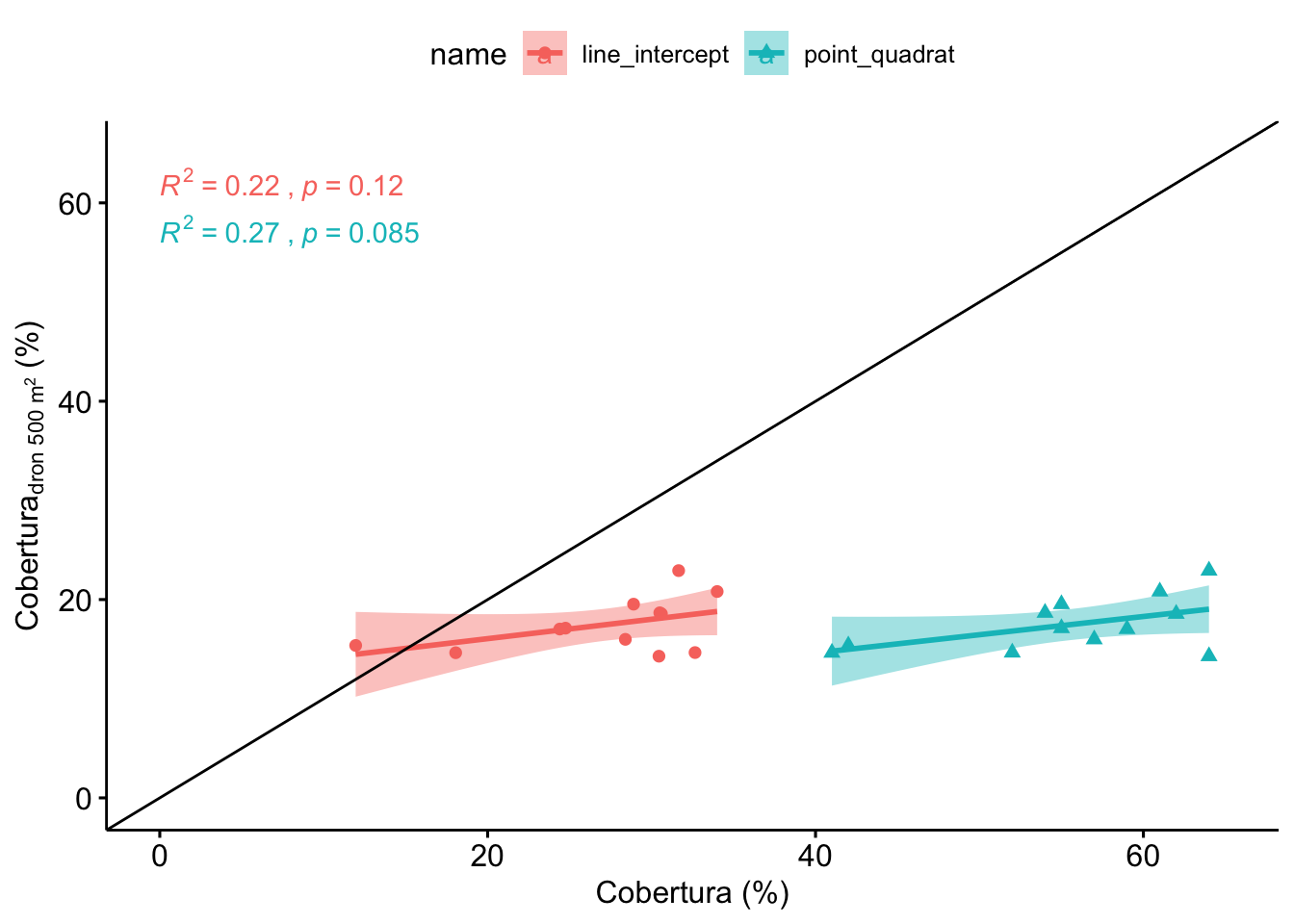
Correlación Quadrat - Dron Q
Ver resultados presentados al congreso forestal
1.2 Correlación de dronT (500 m2) con Line Intercept y PointQuadrat
| Version | Author | Date |
|---|---|---|
| 5a89fea | ajpelu | 2022-04-13 |
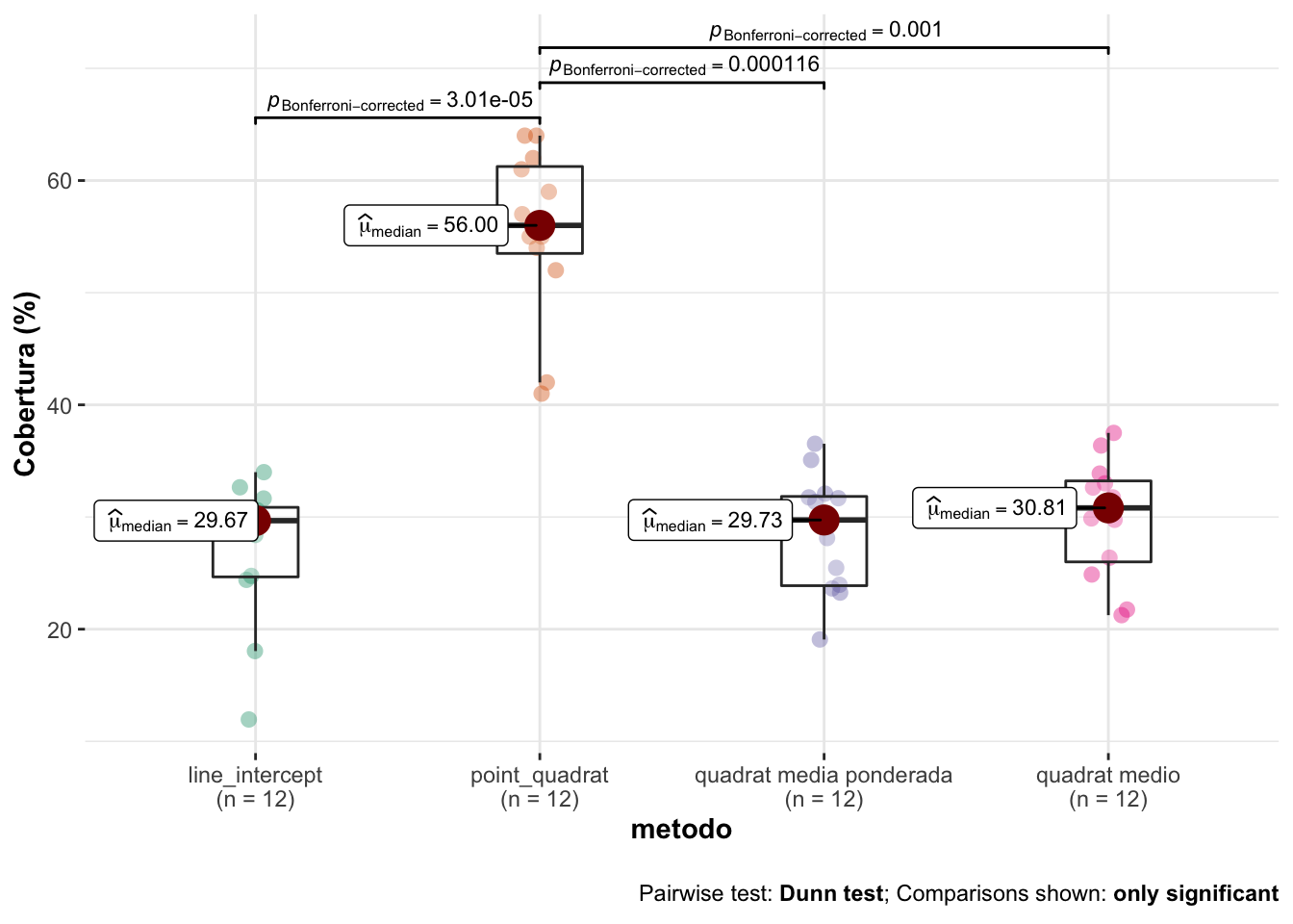
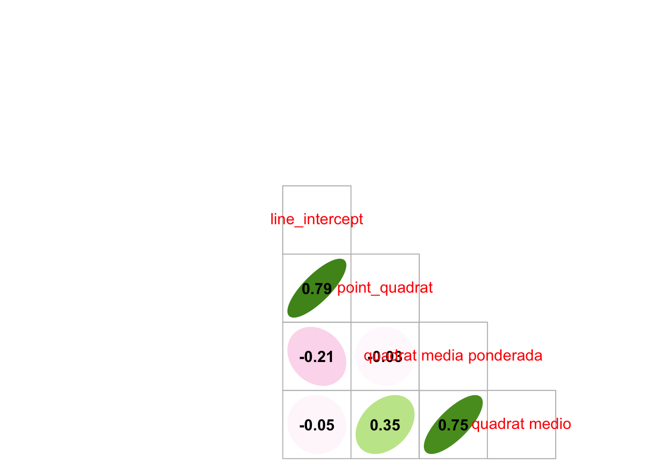
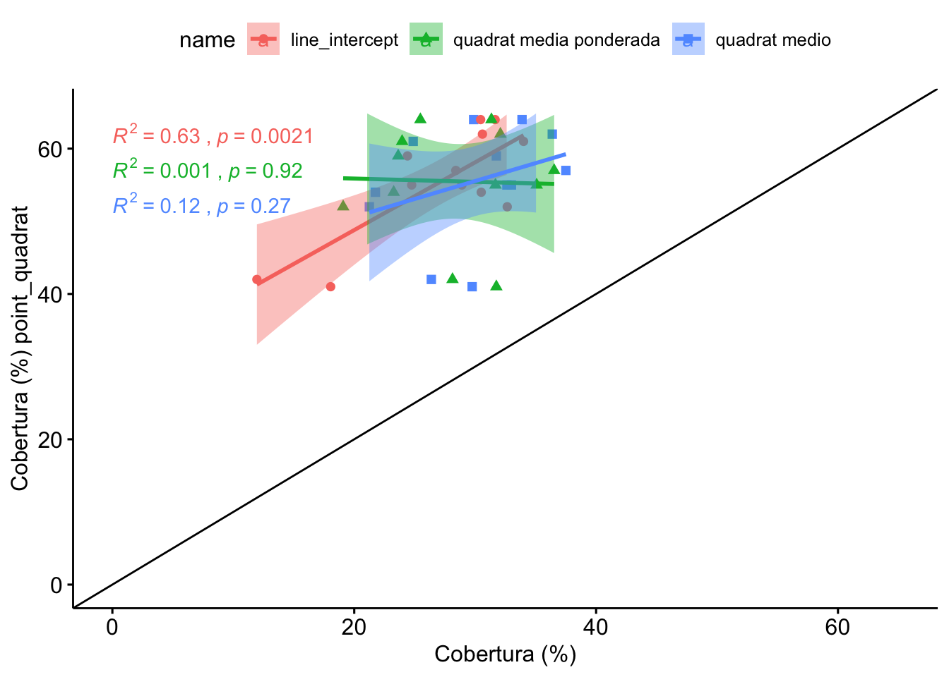
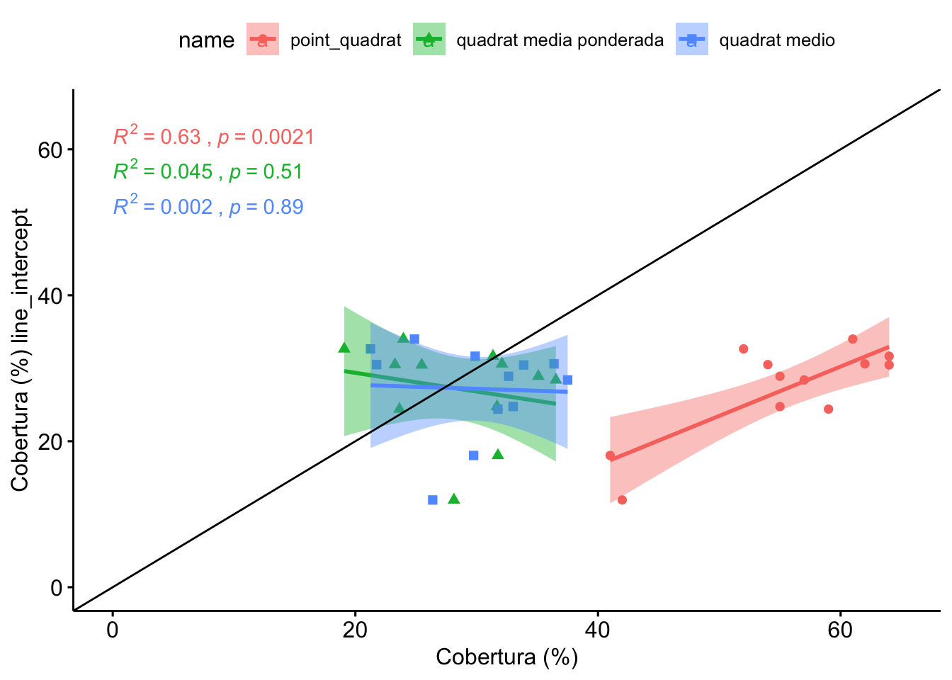
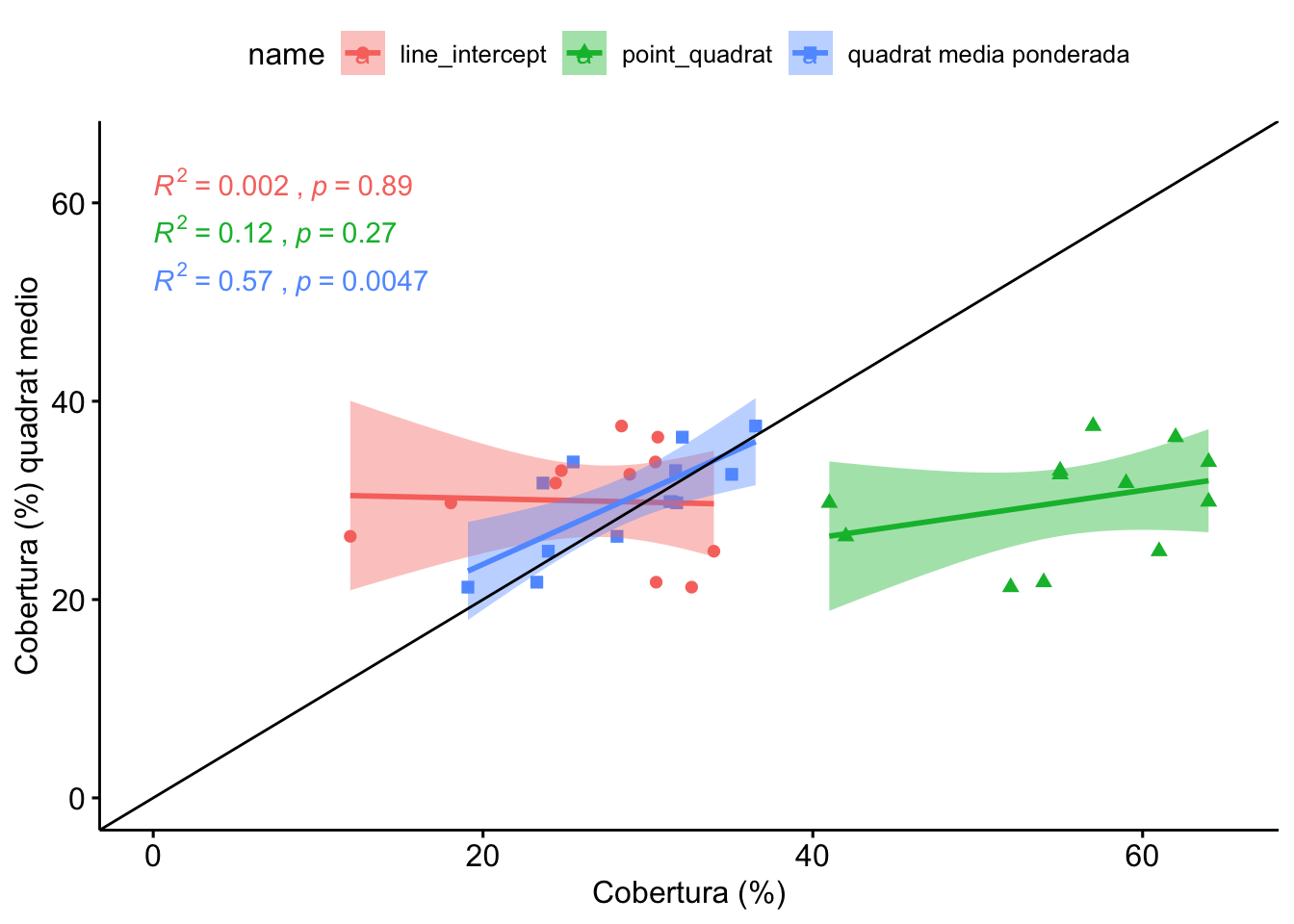
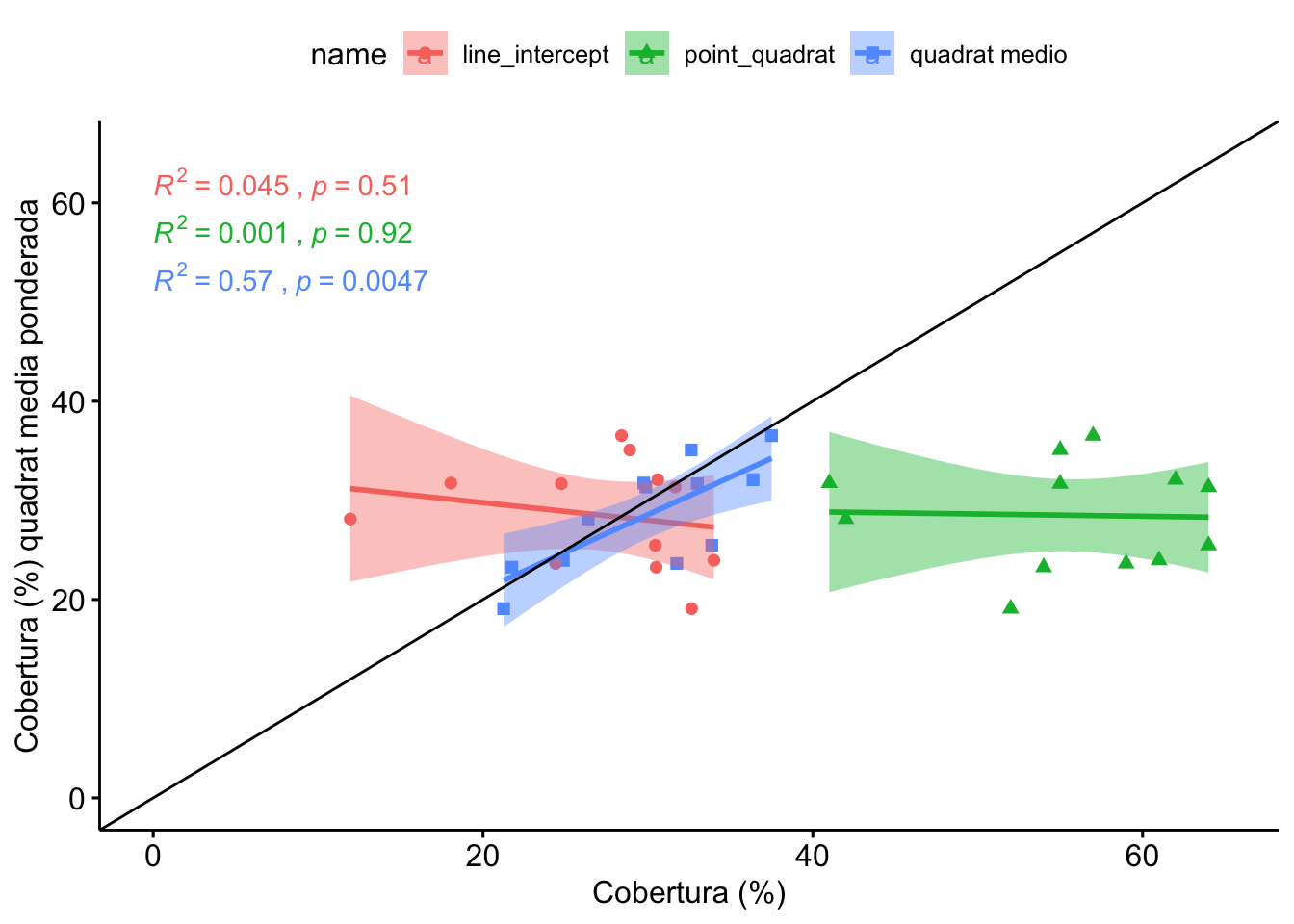
1.3 Comparación Line-Intercept, Quadrat, PointQuadrat
Vamos a realizar la comparación seleccionando para cada parcela (n=12) un valor de cobertura de quadrats. Éste valor se calcula mediante dos aproximaciones:
- Promediando para cada parcela el valor de los quadrats
- Utilizando las medias ponderadas (valores de cobertura de los quadrats ponderados en función de la distribución inicial)
# A tibble: 12 x 3
   parcela  value metodo
   <chr>    <dbl> <chr>
 1 AL_NP_13  36.4 quadrat medio
 2 AL_NP_7   21.8 quadrat medio
 3 AL_NP_8   33   quadrat medio
 4 AL_NP_9   29.9 quadrat medio
 5 AL_P_11   24.9 quadrat medio
 6 AL_P_12   33.9 quadrat medio
 7 AL_P_14   31.8 quadrat medio
 8 AL_P_4    37.5 quadrat medio
 9 AL_PR_15  29.8 quadrat medio
10 AL_PR_16  32.6 quadrat medio
11 AL_PR_17  21.2 quadrat medio
12 AL_PR_18 26.4 quadrat medio| statistic | p.value | parameter | method | mi_variable |
|---|---|---|---|---|
| 27.11094 | 5.6e-06 | 3 | Kruskal-Wallis rank sum test | cobertura |
- Posteriormente computamos las pruebas post-hoc
| H0 | statistic | p.value |
|---|---|---|
| line_intercept = point_quadrat | 4.56 | <0.001 |
| line_intercept = quadrat medio | 0.80 | >0.999 |
| line_intercept = quadrat media ponderada | 0.29 | >0.999 |
| point_quadrat = quadrat medio | 3.76 | 0.001 |
| point_quadrat = quadrat media ponderada | 4.27 | <0.001 |
| quadrat medio = quadrat media ponderada | 0.51 | >0.999 |
| Version | Author | Date |
|---|---|---|
| 5a89fea | ajpelu | 2022-04-13 |
Observamos que no hay diferencias entre LI, y los quadrats medios, ni quadrats ponderado.
Coeficiente de Variación
Analizamos los datos de CV, si son diferentes significativamente. Aplicamos el test MSLRT (Modified signed-likelihood ratio test) para cada uno de los pares de métodos.
| V1 | V2 | MSLRT | p_value |
|---|---|---|---|
| quadrat | dronQ | 6.13 | 0.01326 |
| quadrat | line_intercept | 9.22 | 0.00240 |
| quadrat | point_quadrat | 19.22 | 0.00001 |
| quadrat | dronT | 16.88 | 0.00004 |
| dronQ | line_intercept | 13.98 | 0.00019 |
| dronQ | point_quadrat | 24.60 | 0.00000 |
| dronQ | dronT | 22.16 | 0.00000 |
| line_intercept | point_quadrat | 2.88 | 0.08977 |
| line_intercept | dronT | 1.77 | 0.18398 |
| point_quadrat | dronT | 0.14 | 0.70956 |
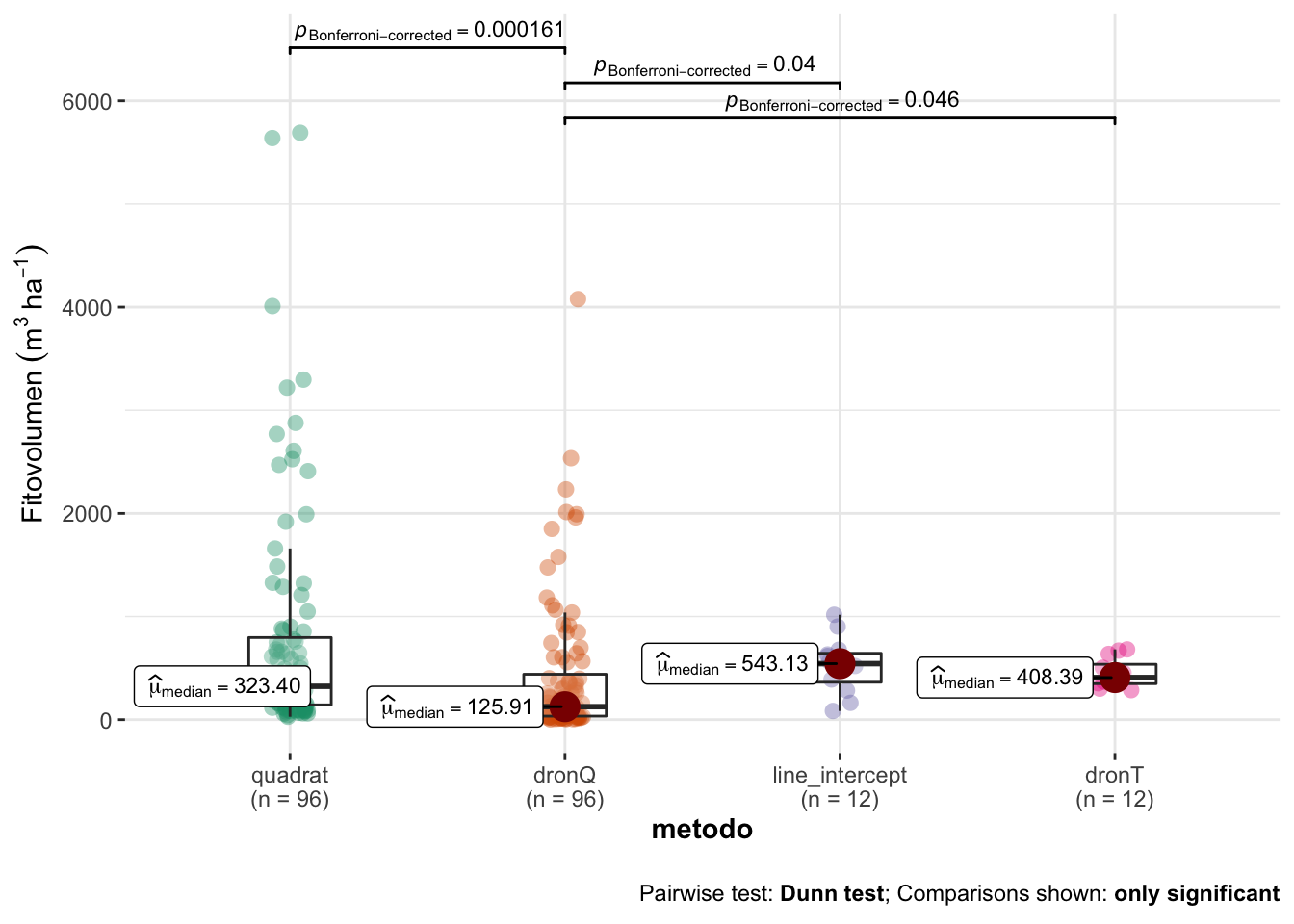
Fitovolumen
- Summary values
| metodo | mean | sd | se | cv | median | n |
|---|---|---|---|---|---|---|
| quadrat | 778.57 | 1108.78 | 113.16 | 142.41 | 323.40 | 96 |
| dronQ | 421.70 | 678.47 | 69.25 | 160.89 | 125.90 | 96 |
| line_intercept | 531.04 | 274.90 | 79.36 | 51.77 | 543.13 | 12 |
| dronT | 450.63 | 141.74 | 40.92 | 31.45 | 408.39 | 12 |
Modelo
- Aplicamos un modelo de Kruskal-Wallis con comparaciones post-hoc aplicando test de Dunn (correcciones de Bonferroni).
- Los resultados son los siguientes:
| statistic | p.value | parameter | method | mi_variable |
|---|---|---|---|---|
| 23.40999 | 3.32e-05 | 3 | Kruskal-Wallis rank sum test | fitovolumen |
- Posteriormente computamos las pruebas post-hoc
| H0 | statistic | p.value |
|---|---|---|
| quadrat = dronQ | 4.20 | 0.0002 |
| quadrat = line_intercept | 0.74 | 1.0000 |
| quadrat = dronT | 0.68 | 1.0000 |
| dronQ = line_intercept | 2.72 | 0.0397 |
| dronQ = dronT | 2.66 | 0.0464 |
| line_intercept = dronT | 0.04 | 1.0000 |
| Version | Author | Date |
|---|---|---|
| 5a89fea | ajpelu | 2022-04-13 |
Coeficiente de Variación
Analizamos los datos de CV, si son diferentes significativamente. Aplicamos el test MSLRT (Modified signed-likelihood ratio test) para cada uno de los pares de métodos.
| V1 | V2 | MSLRT | p_value |
|---|---|---|---|
| quadrat | dronQ | 0.27 | 0.60538 |
| quadrat | line_intercept | 4.69 | 0.03041 |
| quadrat | dronT | 10.28 | 0.00135 |
| dronQ | line_intercept | 4.89 | 0.02694 |
| dronQ | dronT | 9.99 | 0.00158 |
| line_intercept | dronT | 1.94 | 0.16351 |
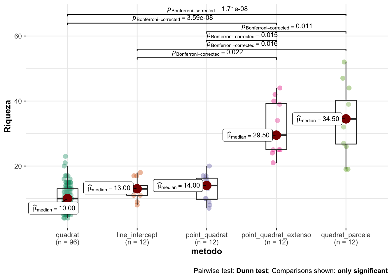
Richness
- Summary values
| metodo | mean | sd | se | cv | median | n |
|---|---|---|---|---|---|---|
| quadrat | 10.57 | 3.89 | 0.40 | 36.77 | 10.0 | 96 |
| line_intercept | 13.00 | 3.10 | 0.90 | 23.88 | 13.0 | 12 |
| point_quadrat | 13.17 | 4.24 | 1.22 | 32.20 | 14.0 | 12 |
| point_quadrat_extenso | 31.50 | 7.99 | 2.31 | 25.38 | 29.5 | 12 |
| quadrat_parcela | 34.08 | 10.39 | 3.00 | 30.48 | 34.5 | 12 |
Modelo
- Aplicamos un modelo de Kruskal-Wallis con comparaciones post-hoc aplicando test de Dunn (correcciones de Bonferroni).
- Los resultados son los siguientes:
| statistic | p.value | parameter | method | mi_variable |
|---|---|---|---|---|
| 64.59165 | 0 | 4 | Kruskal-Wallis rank sum test | riqueza |
- Posteriormente computamos las pruebas post-hoc
| H0 | statistic | p.value |
|---|---|---|
| quadrat = line_intercept | 1.82 | 0.6853 |
| quadrat = point_quadrat | 1.68 | 0.9341 |
| quadrat = point_quadrat_extenso | 5.90 | 0.0000 |
| quadrat = quadrat_parcela | 6.02 | 0.0000 |
| line_intercept = point_quadrat | 0.11 | 1.0000 |
| line_intercept = point_quadrat_extenso | 3.06 | 0.0221 |
| line_intercept = quadrat_parcela | 3.15 | 0.0163 |
| point_quadrat = point_quadrat_extenso | 3.17 | 0.0153 |
| point_quadrat = quadrat_parcela | 3.26 | 0.0112 |
| point_quadrat_extenso = quadrat_parcela | 0.09 | 1.0000 |
| Version | Author | Date |
|---|---|---|
| 5a89fea | ajpelu | 2022-04-13 |
Coeficiente de Variación
Analizamos los datos de CV, si son diferentes significativamente. Aplicamos el test MSLRT (Modified signed-likelihood ratio test) para cada uno de los pares de métodos.
| V1 | V2 | MSLRT | p_value |
|---|---|---|---|
| quadrat | line_intercept | 2.82 | 0.09335 |
| quadrat | point_quadrat | 0.40 | 0.52492 |
| quadrat | point_quadrat_extenso | 2.18 | 0.14018 |
| quadrat | quadrat_parcela | 0.70 | 0.40309 |
| line_intercept | point_quadrat | 0.80 | 0.37022 |
| line_intercept | point_quadrat_extenso | 0.02 | 0.87866 |
| line_intercept | quadrat_parcela | 0.54 | 0.46359 |
| point_quadrat | point_quadrat_extenso | 0.50 | 0.47807 |
| point_quadrat | quadrat_parcela | 0.01 | 0.90371 |
| point_quadrat_extenso | quadrat_parcela | 0.30 | 0.58628 |
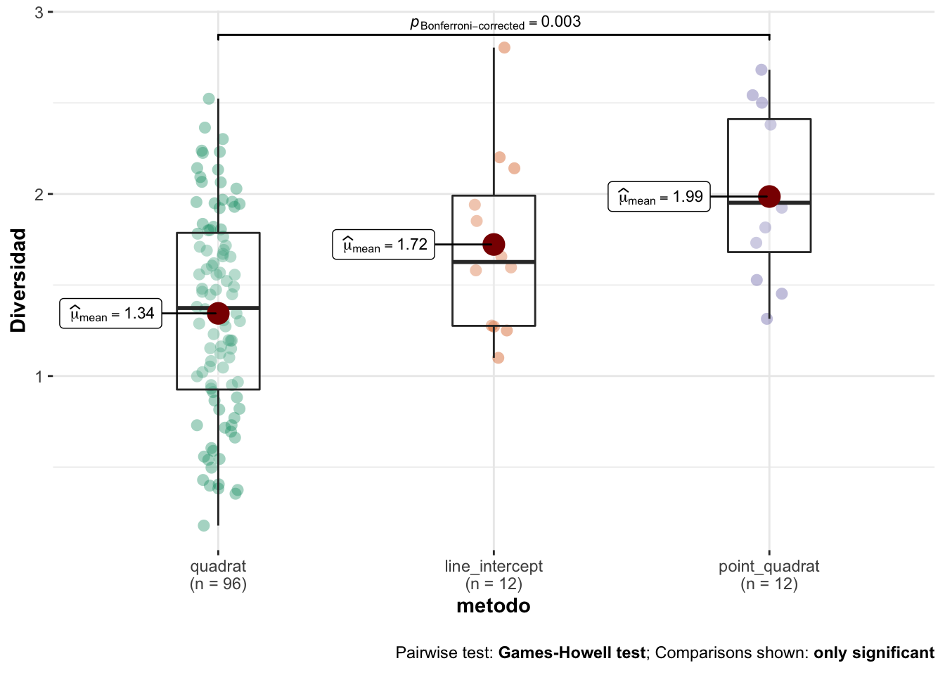
Shannon
- Summary values
| metodo | mean | sd | se | cv | median | n |
|---|---|---|---|---|---|---|
| quadrat | 1.34 | 0.56 | 0.06 | 41.72 | 1.37 | 96 |
| line_intercept | 1.72 | 0.49 | 0.14 | 28.71 | 1.63 | 12 |
| point_quadrat | 1.99 | 0.45 | 0.13 | 22.82 | 1.95 | 12 |
Modelo
- Aplicamos un modelo de ANOVA con comparaciones post-hoc aplicando test de Dunn (correcciones de Bonferroni).
- Los resultados son los siguientes:
OK: There is not clear evidence for different variances across groups (Bartlett Test, p = 0.611).OK: residuals appear as normally distributed (p = 0.168).| Parameter | Sum_Squares | df | Mean_Square | F | p | Eta2 | Eta2_CI_low | Eta2_CI_high |
|---|---|---|---|---|---|---|---|---|
| metodo | 5.41 | 2 | 2.71 | 9.09 | 0.00021 | 0.134 | 0.046 | 0.227 |
| Residuals | 34.83 | 117 | 0.30 |
The ANOVA (formula: value ~ metodo) suggests that:

  - The main effect of metodo is statistically significant and medium (F(2, 117) = 9.09, p < .001; Eta2 = 0.13, 90% CI [0.05, 0.23])

Effect sizes were labelled following Field's (2013) recommendations.- Posteriormente computamos las pruebas post-hoc
| contrast | estimate | SE | df | t.ratio | p.value |
|---|---|---|---|---|---|
| quadrat - line_intercept | -0.378 | 0.167 | 117 | -2.27 | 0.0760 |
| quadrat - point_quadrat | -0.642 | 0.167 | 117 | -3.84 | 0.0006 |
| line_intercept - point_quadrat | -0.263 | 0.223 | 117 | -1.18 | 0.7181 |
| Version | Author | Date |
|---|---|---|
| 5a89fea | ajpelu | 2022-04-13 |
Coeficiente de Variación
Analizamos los datos de CV, si son diferentes significativamente. Aplicamos el test MSLRT (Modified signed-likelihood ratio test) para cada uno de los pares de métodos.
| V1 | V2 | MSLRT | p_value |
|---|---|---|---|
| quadrat | line_intercept | 2.13 | 0.14465 |
| quadrat | point_quadrat | 4.81 | 0.02832 |
| line_intercept | point_quadrat | 0.48 | 0.48795 |
R version 4.0.2 (2020-06-22)
Platform: x86_64-apple-darwin17.0 (64-bit)
Running under: macOS Catalina 10.15.3

Matrix products: default
BLAS:   /Library/Frameworks/R.framework/Versions/4.0/Resources/lib/libRblas.dylib
LAPACK: /Library/Frameworks/R.framework/Versions/4.0/Resources/lib/libRlapack.dylib

locale:
[1] en_US.UTF-8/en_US.UTF-8/en_US.UTF-8/C/en_US.UTF-8/en_US.UTF-8

attached base packages:
[1] stats     graphics  grDevices utils     datasets  methods   base

other attached packages:
 [1] corrplot_0.92      multcompView_0.1-8 ggtext_0.1.1       PMCMRplus_1.9.3
 [5] PMCMR_4.3          statmod_1.4.36     tweedie_2.3.3      report_0.3.0
 [9] kableExtra_1.3.1   cvequality_0.2.0   performance_0.8.0  ggdist_3.0.1
[13] Metrics_0.1.4      ggstatsplot_0.7.2  colorspace_2.0-2   ggpubr_0.4.0
[17] ggforce_0.3.2      ggdark_0.2.1       janitor_2.1.0      here_1.0.1
[21] forcats_0.5.1      stringr_1.4.0      dplyr_1.0.6        purrr_0.3.4
[25] readr_1.4.0        tidyr_1.1.3        tibble_3.1.2       ggplot2_3.3.5
[29] tidyverse_1.3.1    workflowr_1.7.0

loaded via a namespace (and not attached):
  [1] readxl_1.3.1              pairwiseComparisons_3.1.3
  [3] backports_1.2.1           systemfonts_1.0.0
  [5] plyr_1.8.6                splines_4.0.2
  [7] gmp_0.6-2                 kSamples_1.2-9
  [9] ipmisc_5.0.2              TH.data_1.0-10
 [11] digest_0.6.27             SuppDists_1.1-9.5
 [13] htmltools_0.5.2           fansi_0.4.2
 [15] magrittr_2.0.1            memoise_2.0.0
 [17] paletteer_1.3.0           openxlsx_4.2.3
 [19] modelr_0.1.8              sandwich_3.0-0
 [21] rvest_1.0.0               ggrepel_0.9.1
 [23] textshaping_0.3.2         haven_2.3.1
 [25] xfun_0.23                 prismatic_1.0.0
 [27] callr_3.7.0               crayon_1.4.1
 [29] jsonlite_1.7.2            zeallot_0.1.0
 [31] survival_3.2-7            zoo_1.8-8
 [33] glue_1.4.2                polyclip_1.10-0
 [35] gtable_0.3.0              emmeans_1.5.4
 [37] webshot_0.5.2             MatrixModels_0.4-1
 [39] distributional_0.3.0      statsExpressions_1.1.0
 [41] car_3.0-10                Rmpfr_0.8-2
 [43] abind_1.4-5               scales_1.1.1.9000
 [45] mvtnorm_1.1-1             DBI_1.1.1
 [47] rstatix_0.6.0             Rcpp_1.0.7
 [49] gridtext_0.1.4            viridisLite_0.4.0
 [51] xtable_1.8-4              foreign_0.8-81
 [53] httr_1.4.2                ellipsis_0.3.2
 [55] pkgconfig_2.0.3           reshape_0.8.8
 [57] farver_2.1.0              sass_0.3.1
 [59] dbplyr_2.1.1              utf8_1.1.4
 [61] labeling_0.4.2            effectsize_0.4.5
 [63] tidyselect_1.1.1          rlang_0.4.12
 [65] later_1.1.0.1             ggcorrplot_0.1.3
 [67] munsell_0.5.0             cellranger_1.1.0
 [69] tools_4.0.2               cachem_1.0.4
 [71] cli_2.5.0                 generics_0.1.0
 [73] broom_0.7.9               evaluate_0.14
 [75] fastmap_1.1.0             ragg_1.1.1
 [77] BWStest_0.2.2             yaml_2.2.1
 [79] rematch2_2.1.2            processx_3.5.1
 [81] knitr_1.31                fs_1.5.0
 [83] zip_2.1.1                 nlme_3.1-152
 [85] WRS2_1.1-1                pbapply_1.4-3
 [87] whisker_0.4               xml2_1.3.2
 [89] correlation_0.6.1         compiler_4.0.2
 [91] rstudioapi_0.13           curl_4.3
 [93] ggsignif_0.6.0            reprex_2.0.0
 [95] tweenr_1.0.1              bslib_0.2.4
 [97] stringi_1.7.4             highr_0.8
 [99] ps_1.5.0                  parameters_0.14.0
[101] lattice_0.20-41           Matrix_1.3-2
[103] vctrs_0.3.8               pillar_1.6.1
[105] lifecycle_1.0.1           mc2d_0.1-18
[107] jquerylib_0.1.3           estimability_1.3
[109] data.table_1.14.0         insight_0.14.4
[111] patchwork_1.1.1           httpuv_1.5.5
[113] R6_2.5.1                  promises_1.2.0.1
[115] rio_0.5.16                BayesFactor_0.9.12-4.2
[117] codetools_0.2-18          MASS_7.3-53
[119] gtools_3.8.2              assertthat_0.2.1
[121] rprojroot_2.0.2           withr_2.4.1
[123] multcomp_1.4-16           mgcv_1.8-33
[125] bayestestR_0.9.0          parallel_4.0.2
[127] hms_1.0.0                 grid_4.0.2
[129] coda_0.19-4               rmarkdown_2.8
[131] snakecase_0.11.0          carData_3.0-4
[133] git2r_0.28.0              getPass_0.2-2
[135] lubridate_1.7.10