Pre- and post-fire anaylisis of soils
Last updated: 2022-02-17
Checks: 6 1
Knit directory: soil_alcontar/
This reproducible R Markdown analysis was created with workflowr (version 1.7.0). The Checks tab describes the reproducibility checks that were applied when the results were created. The Past versions tab lists the development history.
Great! Since the R Markdown file has been committed to the Git repository, you know the exact version of the code that produced these results.
Great job! The global environment was empty. Objects defined in the global environment can affect the analysis in your R Markdown file in unknown ways. For reproduciblity it’s best to always run the code in an empty environment.
The command set.seed(20210907) was run prior to running the code in the R Markdown file. Setting a seed ensures that any results that rely on randomness, e.g. subsampling or permutations, are reproducible.
Great job! Recording the operating system, R version, and package versions is critical for reproducibility.
- pkgs
- prepare-data
- session-info-chunk-inserted-by-workflowr
- unnamed-chunk-1
- unnamed-chunk-10
- unnamed-chunk-11
- unnamed-chunk-12
- unnamed-chunk-13
- unnamed-chunk-14
- unnamed-chunk-15
- unnamed-chunk-16
- unnamed-chunk-17
- unnamed-chunk-18
- unnamed-chunk-19
- unnamed-chunk-2
- unnamed-chunk-20
- unnamed-chunk-21
- unnamed-chunk-22
- unnamed-chunk-23
- unnamed-chunk-24
- unnamed-chunk-25
- unnamed-chunk-26
- unnamed-chunk-27
- unnamed-chunk-28
- unnamed-chunk-29
- unnamed-chunk-3
- unnamed-chunk-30
- unnamed-chunk-31
- unnamed-chunk-32
- unnamed-chunk-33
- unnamed-chunk-34
- unnamed-chunk-35
- unnamed-chunk-36
- unnamed-chunk-37
- unnamed-chunk-38
- unnamed-chunk-39
- unnamed-chunk-4
- unnamed-chunk-40
- unnamed-chunk-41
- unnamed-chunk-42
- unnamed-chunk-43
- unnamed-chunk-44
- unnamed-chunk-45
- unnamed-chunk-46
- unnamed-chunk-47
- unnamed-chunk-48
- unnamed-chunk-49
- unnamed-chunk-5
- unnamed-chunk-50
- unnamed-chunk-51
- unnamed-chunk-52
- unnamed-chunk-53
- unnamed-chunk-54
- unnamed-chunk-55
- unnamed-chunk-56
- unnamed-chunk-57
- unnamed-chunk-58
- unnamed-chunk-59
- unnamed-chunk-6
- unnamed-chunk-60
- unnamed-chunk-61
- unnamed-chunk-62
- unnamed-chunk-63
- unnamed-chunk-64
- unnamed-chunk-65
- unnamed-chunk-66
- unnamed-chunk-67
- unnamed-chunk-68
- unnamed-chunk-69
- unnamed-chunk-7
- unnamed-chunk-70
- unnamed-chunk-71
- unnamed-chunk-72
- unnamed-chunk-73
- unnamed-chunk-74
- unnamed-chunk-75
- unnamed-chunk-76
- unnamed-chunk-8
- unnamed-chunk-9
To ensure reproducibility of the results, delete the cache directory analysis_pre_post_cache and re-run the analysis. To have workflowr automatically delete the cache directory prior to building the file, set delete_cache = TRUE when running wflow_build() or wflow_publish().
Great job! Using relative paths to the files within your workflowr project makes it easier to run your code on other machines.
Great! You are using Git for version control. Tracking code development and connecting the code version to the results is critical for reproducibility.
The results in this page were generated with repository version 8960975. See the Past versions tab to see a history of the changes made to the R Markdown and HTML files.
Note that you need to be careful to ensure that all relevant files for the analysis have been committed to Git prior to generating the results (you can use wflow_publish or wflow_git_commit). workflowr only checks the R Markdown file, but you know if there are other scripts or data files that it depends on. Below is the status of the Git repository when the results were generated:
Ignored files:
    Ignored:    .RData
    Ignored:    .Rhistory
    Ignored:    .Rproj.user/C369E4F4/
    Ignored:    .Rproj.user/shared/notebooks/0EF54E14-NOBORRAR/
    Ignored:    .Rproj.user/shared/notebooks/27FF967E-analysis_pre_post_epoca/
    Ignored:    .Rproj.user/shared/notebooks/33E25F73-analysis_resilience/
    Ignored:    .Rproj.user/shared/notebooks/3F603CAC-map/
    Ignored:    .Rproj.user/shared/notebooks/4672E36C-study_area/
    Ignored:    .Rproj.user/shared/notebooks/4A68381F-general_overview_soils/
    Ignored:    .Rproj.user/shared/notebooks/4E13660A-temporal_comparison/
    Ignored:    .Rproj.user/shared/notebooks/5D919DFD-analysis_zona_time_postFire/
    Ignored:    .Rproj.user/shared/notebooks/827D0727-analysis_pre_post/
    Ignored:    .Rproj.user/shared/notebooks/A3F813C2-index/
    Ignored:    .Rproj.user/shared/notebooks/D4E3AA10-analysis_zona_time/

Untracked files:
    Untracked:  analysis/NOBORRAR.Rmd
    Untracked:  analysis/analysis_pre_post_cache/
    Untracked:  analysis/test.Rmd
    Untracked:  data/spatial/lucdeme/
    Untracked:  data/spatial/test/
    Untracked:  map.Rmd
    Untracked:  output/anovas_pre_post_epoca.csv
    Untracked:  output/anovas_zona_time.csv
    Untracked:  output/anovas_zona_time_postFire.csv
    Untracked:  output/meanboot_pre_post_epoca.csv
    Untracked:  scripts/generate_3dview.R

Unstaged changes:
    Modified:   analysis/_site.yml
    Modified:   data/Resultados_Suelos_2018_2021_v2.xlsx
    Modified:   data/spatial/.DS_Store
    Modified:   data/spatial/01_EP_ANDALUCIA/EP_Andalucía.dbf
    Deleted:    index.Rmd
    Modified:   output/anovas_pre_post.csv
    Modified:   scripts/00_prepare_data.R
    Modified:   temporal_comparison.Rmd
Note that any generated files, e.g. HTML, png, CSS, etc., are not included in this status report because it is ok for generated content to have uncommitted changes.
These are the previous versions of the repository in which changes were made to the R Markdown (analysis/analysis_pre_post.Rmd) and HTML (docs/analysis_pre_post.html) files. If you’ve configured a remote Git repository (see ?wflow_git_remote), click on the hyperlinks in the table below to view the files as they were in that past version.
| File | Version | Author | Date | Message |
|---|---|---|---|---|
| html | eadc8da | ajpelu | 2021-09-14 | Build site. |
| Rmd | ecb1e66 | ajpelu | 2021-09-14 | generate analysis with new data nh4 |
| html | 71c36dd | ajpelu | 2021-09-10 | Build site. |
| Rmd | 297463f | ajpelu | 2021-09-10 | add anova tables; remove preeliminar homedasticity |
| html | 46f8fd8 | ajpelu | 2021-09-07 | Build site. |
| Rmd | 2c59a9d | ajpelu | 2021-09-07 | update |
| html | 68358ce | ajpelu | 2021-09-07 | Build site. |
| Rmd | 6ef970d | ajpelu | 2021-09-07 | add plot |
| html | bfa8071 | ajpelu | 2021-09-07 | Build site. |
| Rmd | dc87911 | ajpelu | 2021-09-07 | include pre post analysis |
Prepare data
raw_soil <- readxl::read_excel(here::here("data/Resultados_Suelos_2018_2021_v2.xlsx"),
    sheet = "SEGUIMIENTO_SUELOS_sin_ouliers") %>% janitor::clean_names() %>% mutate(treatment_name = case_when(str_detect(geo_parcela_nombre,
    "NP_") ~ "Autumn Burning / No Browsing", str_detect(geo_parcela_nombre, "PR_") ~
    "Spring Burning / Browsing", str_detect(geo_parcela_nombre, "P_") ~ "Autumn Burning / Browsing"),
    zona = case_when(str_detect(geo_parcela_nombre, "NP_") ~ "QOt_NP", str_detect(geo_parcela_nombre,
        "PR_") ~ "QPr_P", str_detect(geo_parcela_nombre, "P_") ~ "QOt_P"), fecha = lubridate::ymd(fecha),
    pre_post_quema = case_when(pre_post_quema == "Prequema" ~ "0 preQuema", pre_post_quema ==
"Postquema" ~ "1 postQuema"))- Select data pre- and intermediately post-fire (first post-fire sampling: “2018-12-20” and “2019-05-09” for autumn and spring fires respectively)
soil <- raw_soil %>% filter(fecha %in% lubridate::ymd(c("2018-12-11", "2018-12-20",
"2019-04-24", "2019-05-09"))) %>% mutate(zona = as.factor(zona), pre_post_quema = as.factor(pre_post_quema))- Structure of the data
              zona
pre_post_quema QOt_NP QOt_P QPr_P
   0 preQuema      24    24    24
   1 postQuema     24    24    24
Modelize
- For each response variable, the approach modelling is
\(Y \sim zona (P|NP|PR) + Fecha(pre|post) + zona \times Fecha\)
using the “(1|zona:geo_parcela_nombre)” as nested random effects
Then explore error distribution of the variable response and model diagnostics
Select the appropiate error distribution and use LMM or GLMM
Explore Post-hoc
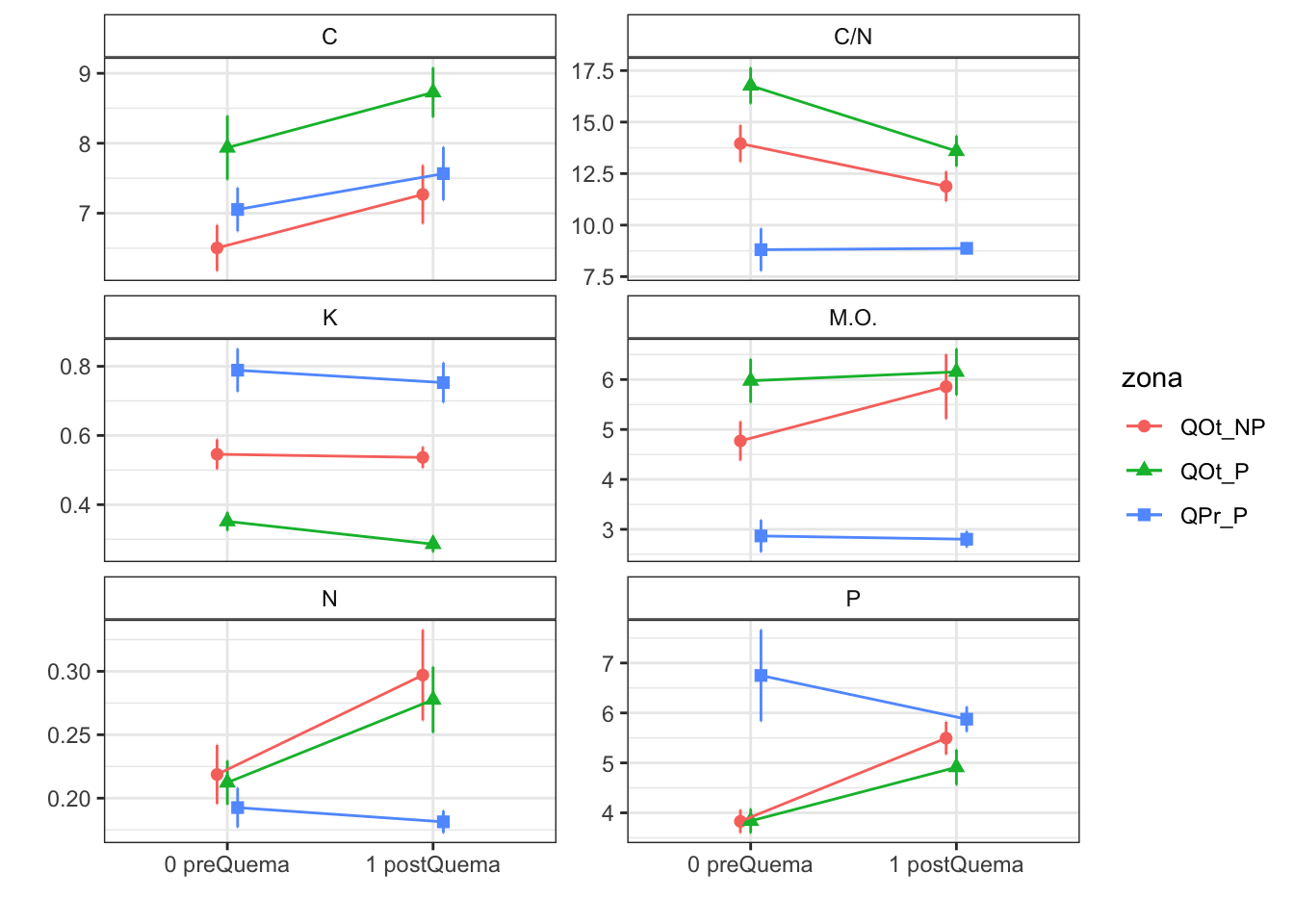
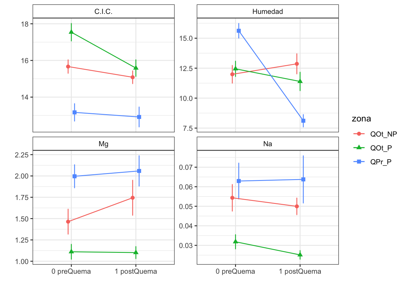
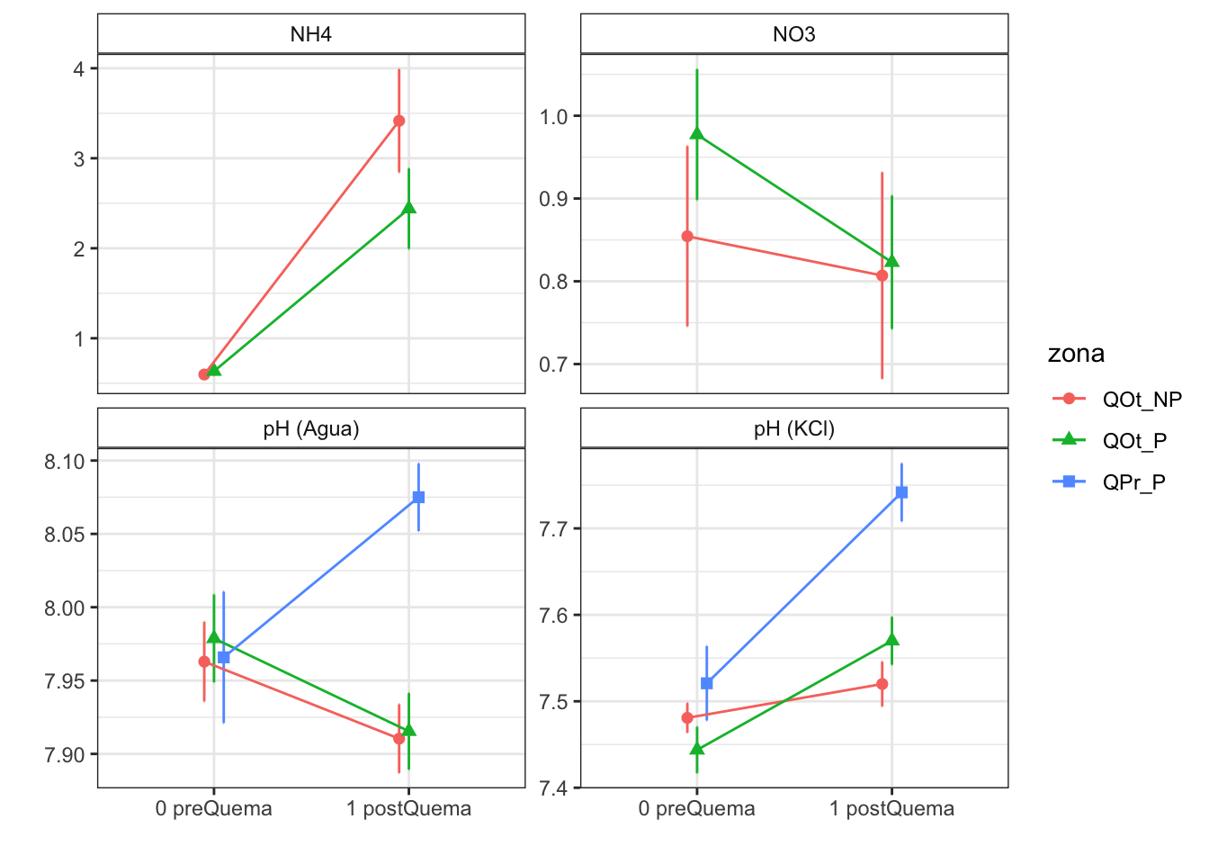
Plot interactions
Humedad
Model
Type III Analysis of Variance Table with Satterthwaite's method
                    Sum Sq Mean Sq NumDF DenDF F value    Pr(>F)
pre_post_quema      236.42 236.416     1   129 26.1050 1.136e-06 ***
zona                  1.46   0.728     2     9  0.0803    0.9235
pre_post_quema:zona 462.22 231.109     2   129 25.5190 4.593e-10 ***
---
Signif. codes:  0 '***' 0.001 '**' 0.01 '*' 0.05 '.' 0.1 ' ' 1
Sum Sq Mean Sq NumDF DenDF F value Pr(>F)
pre_post_quema 236.415514 236.4155136 1 129 26.10495006 1.135929e-06
zona 1.455293 0.7276463 2 9 0.08034655 9.234509e-01
pre_post_quema:zona 462.217132 231.1085659 2 129 25.51895804 4.592612e-10
variable factor
pre_post_quema humedad pre_post_quema
zona humedad zona
pre_post_quema:zona humedad pre_post_quema:zonaPost-hoc
$`emmeans of pre_post_quema`
 pre_post_quema emmean    SE   df lower.CL upper.CL
 0 preQuema       13.4 0.676 12.1    11.88     14.8
 1 postQuema      10.8 0.676 12.1     9.32     12.3

Results are averaged over the levels of: zona
Degrees-of-freedom method: kenward-roger
Confidence level used: 0.95

$`pairwise differences of pre_post_quema`
 1                        estimate    SE  df t.ratio p.value
 0 preQuema - 1 postQuema     2.56 0.502 129 5.109   <.0001

Results are averaged over the levels of: zona
Degrees-of-freedom method: kenward-roger
$`emmeans of zona`
zona emmean SE df lower.CL upper.CL
QOt_NP 12.4 1.09 9 9.97 14.9
QOt_P 11.9 1.09 9 9.46 14.4
QPr_P 11.9 1.09 9 9.41 14.3
Results are averaged over the levels of: pre_post_quema
Degrees-of-freedom method: kenward-roger
Confidence level used: 0.95
$`pairwise differences of zona`
1 estimate SE df t.ratio p.value
QOt_NP - QOt_P 0.5060 1.54 9 0.329 0.9424
QOt_NP - QPr_P 0.5579 1.54 9 0.363 0.9306
QOt_P - QPr_P 0.0518 1.54 9 0.034 0.9994
Results are averaged over the levels of: pre_post_quema
Degrees-of-freedom method: kenward-roger
P value adjustment: tukey method for comparing a family of 3 estimates $`emmeans of pre_post_quema | zona`
zona = QOt_NP:
pre_post_quema emmean SE df lower.CL upper.CL
0 preQuema 11.99 1.17 12.1 9.44 14.5
1 postQuema 12.86 1.17 12.1 10.31 15.4
zona = QOt_P:
pre_post_quema emmean SE df lower.CL upper.CL
0 preQuema 12.45 1.17 12.1 9.90 15.0
1 postQuema 11.39 1.17 12.1 8.84 13.9
zona = QPr_P:
pre_post_quema emmean SE df lower.CL upper.CL
0 preQuema 15.62 1.17 12.1 13.07 18.2
1 postQuema 8.11 1.17 12.1 5.57 10.7
Degrees-of-freedom method: kenward-roger
Confidence level used: 0.95
$`pairwise differences of pre_post_quema | zona`
zona = QOt_NP:
2 estimate SE df t.ratio p.value
0 preQuema - 1 postQuema -0.872 0.869 129 -1.004 0.3171
zona = QOt_P:
2 estimate SE df t.ratio p.value
0 preQuema - 1 postQuema 1.054 0.869 129 1.213 0.2273
zona = QPr_P:
2 estimate SE df t.ratio p.value
0 preQuema - 1 postQuema 7.507 0.869 129 8.641 <.0001
Degrees-of-freedom method: kenward-roger CIC
Model
Type III Analysis of Variance Table with Satterthwaite's method
                    Sum Sq Mean Sq NumDF DenDF F value   Pr(>F)
pre_post_quema      31.174 31.1736     1   129  8.7568 0.003671 **
zona                40.297 20.1484     2     9  5.6598 0.025614 *
pre_post_quema:zona 19.681  9.8403     2   129  2.7642 0.066764 .
---
Signif. codes:  0 '***' 0.001 '**' 0.01 '*' 0.05 '.' 0.1 ' ' 1
Sum Sq Mean Sq NumDF DenDF F value Pr(>F)
pre_post_quema 31.17361 31.173609 1 129 8.756838 0.003670913
zona 40.29686 20.148428 2 9 5.659804 0.025613698
pre_post_quema:zona 19.68056 9.840278 2 129 2.764188 0.066763596
variable factor
pre_post_quema cic pre_post_quema
zona cic zona
pre_post_quema:zona cic pre_post_quema:zonaPost-hoc
$`emmeans of pre_post_quema`
 pre_post_quema emmean    SE   df lower.CL upper.CL
 0 preQuema       15.5 0.462 11.5     14.4     16.5
 1 postQuema      14.5 0.462 11.5     13.5     15.5

Results are averaged over the levels of: zona
Degrees-of-freedom method: kenward-roger
Confidence level used: 0.95

$`pairwise differences of pre_post_quema`
 1                        estimate    SE  df t.ratio p.value
 0 preQuema - 1 postQuema    0.931 0.314 129 2.959   0.0037

Results are averaged over the levels of: zona
Degrees-of-freedom method: kenward-roger
$`emmeans of zona`
zona emmean SE df lower.CL upper.CL
QOt_NP 15.4 0.753 9 13.7 17.1
QOt_P 16.6 0.753 9 14.9 18.3
QPr_P 13.0 0.753 9 11.3 14.7
Results are averaged over the levels of: pre_post_quema
Degrees-of-freedom method: kenward-roger
Confidence level used: 0.95
$`pairwise differences of zona`
1 estimate SE df t.ratio p.value
QOt_NP - QOt_P -1.19 1.06 9 -1.115 0.5291
QOt_NP - QPr_P 2.33 1.06 9 2.191 0.1262
QOt_P - QPr_P 3.52 1.06 9 3.307 0.0225
Results are averaged over the levels of: pre_post_quema
Degrees-of-freedom method: kenward-roger
P value adjustment: tukey method for comparing a family of 3 estimates $`emmeans of pre_post_quema | zona`
zona = QOt_NP:
pre_post_quema emmean SE df lower.CL upper.CL
0 preQuema 15.7 0.801 11.5 13.9 17.4
1 postQuema 15.1 0.801 11.5 13.3 16.8
zona = QOt_P:
pre_post_quema emmean SE df lower.CL upper.CL
0 preQuema 17.5 0.801 11.5 15.8 19.3
1 postQuema 15.6 0.801 11.5 13.8 17.3
zona = QPr_P:
pre_post_quema emmean SE df lower.CL upper.CL
0 preQuema 13.2 0.801 11.5 11.4 14.9
1 postQuema 12.9 0.801 11.5 11.2 14.7
Degrees-of-freedom method: kenward-roger
Confidence level used: 0.95
$`pairwise differences of pre_post_quema | zona`
zona = QOt_NP:
2 estimate SE df t.ratio p.value
0 preQuema - 1 postQuema 0.583 0.545 129 1.071 0.2862
zona = QOt_P:
2 estimate SE df t.ratio p.value
0 preQuema - 1 postQuema 1.958 0.545 129 3.595 0.0005
zona = QPr_P:
2 estimate SE df t.ratio p.value
0 preQuema - 1 postQuema 0.250 0.545 129 0.459 0.6470
Degrees-of-freedom method: kenward-roger C
Model
Type III Analysis of Variance Table with Satterthwaite's method
                     Sum Sq Mean Sq NumDF DenDF F value   Pr(>F)
pre_post_quema      17.1120 17.1120     1   129  7.8770 0.005784 **
zona                 5.3708  2.6854     2     9  1.2361 0.335481
pre_post_quema:zona  0.5673  0.2837     2   129  0.1306 0.877707
---
Signif. codes:  0 '***' 0.001 '**' 0.01 '*' 0.05 '.' 0.1 ' ' 1
Sum Sq Mean Sq NumDF DenDF F value Pr(>F)
pre_post_quema 17.1120115 17.112011 1 129 7.8770265 0.00578378
zona 5.3707569 2.685378 2 9 1.2361374 0.33548133
pre_post_quema:zona 0.5673181 0.283659 2 129 0.1305743 0.87770709
variable factor
pre_post_quema c_percent pre_post_quema
zona c_percent zona
pre_post_quema:zona c_percent pre_post_quema:zonaPost-hoc
$`emmeans of pre_post_quema`
 pre_post_quema emmean    SE   df lower.CL upper.CL
 0 preQuema       7.16 0.405 10.9     6.27     8.06
 1 postQuema      7.85 0.405 10.9     6.96     8.75

Results are averaged over the levels of: zona
Degrees-of-freedom method: kenward-roger
Confidence level used: 0.95

$`pairwise differences of pre_post_quema`
 1                        estimate    SE  df t.ratio p.value
 0 preQuema - 1 postQuema   -0.689 0.246 129 -2.807  0.0058

Results are averaged over the levels of: zona
Degrees-of-freedom method: kenward-roger
$`emmeans of zona`
zona emmean SE df lower.CL upper.CL
QOt_NP 6.89 0.669 9 5.37 8.40
QOt_P 8.33 0.669 9 6.82 9.84
QPr_P 7.31 0.669 9 5.80 8.82
Results are averaged over the levels of: pre_post_quema
Degrees-of-freedom method: kenward-roger
Confidence level used: 0.95
$`pairwise differences of zona`
1 estimate SE df t.ratio p.value
QOt_NP - QOt_P -1.446 0.945 9 -1.529 0.3233
QOt_NP - QPr_P -0.424 0.945 9 -0.448 0.8965
QOt_P - QPr_P 1.022 0.945 9 1.081 0.5483
Results are averaged over the levels of: pre_post_quema
Degrees-of-freedom method: kenward-roger
P value adjustment: tukey method for comparing a family of 3 estimates $`emmeans of pre_post_quema | zona`
zona = QOt_NP:
pre_post_quema emmean SE df lower.CL upper.CL
0 preQuema 6.50 0.702 10.9 4.96 8.05
1 postQuema 7.27 0.702 10.9 5.72 8.81
zona = QOt_P:
pre_post_quema emmean SE df lower.CL upper.CL
0 preQuema 7.94 0.702 10.9 6.39 9.48
1 postQuema 8.73 0.702 10.9 7.18 10.27
zona = QPr_P:
pre_post_quema emmean SE df lower.CL upper.CL
0 preQuema 7.05 0.702 10.9 5.51 8.60
1 postQuema 7.57 0.702 10.9 6.02 9.11
Degrees-of-freedom method: kenward-roger
Confidence level used: 0.95
$`pairwise differences of pre_post_quema | zona`
zona = QOt_NP:
2 estimate SE df t.ratio p.value
0 preQuema - 1 postQuema -0.765 0.425 129 -1.799 0.0744
zona = QOt_P:
2 estimate SE df t.ratio p.value
0 preQuema - 1 postQuema -0.790 0.425 129 -1.858 0.0655
zona = QPr_P:
2 estimate SE df t.ratio p.value
0 preQuema - 1 postQuema -0.512 0.425 129 -1.205 0.2306
Degrees-of-freedom method: kenward-roger Fe
Model
Fitting one lmer() model. [DONE]
Calculating p-values. [DONE]
Mixed Model Anova Table (Type 3 tests, KR-method)
Model: fe_percent ~ pre_post_quema * zona + (1 | zona:geo_parcela_nombre)
Data: df_model
Effect df F p.value
1 pre_post_quema 1, 129 0.52 .473
2 zona 2, 9 0.69 .526
3 pre_post_quema:zona 2, 129 0.17 .845
---
Signif. codes: 0 '***' 0.001 '**' 0.01 '*' 0.05 '+' 0.1 ' ' 1Fitting one lmer() model. [DONE]
Calculating p-values. [DONE]Mixed Model Anova Table (Type 3 tests, KR-method)
Model: fe_percent ~ pre_post_quema * zona + (1 | zona:geo_parcela_nombre)
Data: df_model
num Df den Df F Pr(>F)
pre_post_quema 1 129 0.5186 0.4727
zona 2 9 0.6903 0.5261
pre_post_quema:zona 2 129 0.1688 0.8449Post-hoc
$`emmeans of pre_post_quema`
pre_post_quema emmean SE df asymp.LCL asymp.UCL
0 preQuema 0.549 0.00599 Inf 0.537 0.561
1 postQuema 0.560 0.00818 Inf 0.544 0.576
Results are averaged over the levels of: zona
Results are given on the inverse (not the response) scale.
Confidence level used: 0.95
$`pairwise differences of pre_post_quema`
1 estimate SE df z.ratio p.value
0 preQuema - 1 postQuema -0.0112 0.00566 Inf -1.979 0.0478
Results are averaged over the levels of: zona
Note: contrasts are still on the inverse scale $`emmeans of zona`
zona emmean SE df asymp.LCL asymp.UCL
QOt_NP 0.526 0.00599 Inf 0.514 0.538
QOt_P 0.607 0.00848 Inf 0.590 0.623
QPr_P 0.531 0.00846 Inf 0.514 0.547
Results are averaged over the levels of: pre_post_quema
Results are given on the inverse (not the response) scale.
Confidence level used: 0.95
$`pairwise differences of zona`
1 estimate SE df z.ratio p.value
QOt_NP - QOt_P -0.08067 0.00609 Inf -13.241 <.0001
QOt_NP - QPr_P -0.00486 0.00608 Inf -0.799 0.7036
QOt_P - QPr_P 0.07581 0.00860 Inf 8.819 <.0001
Results are averaged over the levels of: pre_post_quema
Note: contrasts are still on the inverse scale
P value adjustment: tukey method for comparing a family of 3 estimates $`emmeans of pre_post_quema | zona`
zona = QOt_NP:
pre_post_quema emmean SE df asymp.LCL asymp.UCL
0 preQuema 0.515 0.00543 Inf 0.504 0.526
1 postQuema 0.537 0.00747 Inf 0.522 0.552
zona = QOt_P:
pre_post_quema emmean SE df asymp.LCL asymp.UCL
0 preQuema 0.601 0.00768 Inf 0.586 0.616
1 postQuema 0.612 0.01058 Inf 0.591 0.633
zona = QPr_P:
pre_post_quema emmean SE df asymp.LCL asymp.UCL
0 preQuema 0.530 0.00767 Inf 0.515 0.545
1 postQuema 0.531 0.01054 Inf 0.511 0.552
Results are given on the inverse (not the response) scale.
Confidence level used: 0.95
$`pairwise differences of pre_post_quema | zona`
zona = QOt_NP:
2 estimate SE df z.ratio p.value
0 preQuema - 1 postQuema -0.02193 0.00519 Inf -4.225 <.0001
zona = QOt_P:
2 estimate SE df z.ratio p.value
0 preQuema - 1 postQuema -0.01062 0.00737 Inf -1.442 0.1493
zona = QPr_P:
2 estimate SE df z.ratio p.value
0 preQuema - 1 postQuema -0.00106 0.00732 Inf -0.144 0.8853
Note: contrasts are still on the inverse scale MO
Model
Fitting one lmer() model. [DONE]
Calculating p-values. [DONE]
Mixed Model Anova Table (Type 3 tests, KR-method)
Model: mo ~ pre_post_quema * zona + (1 | zona:geo_parcela_nombre)
Data: df_model
Effect df F p.value
1 pre_post_quema 1, 129 1.35 .247
2 zona 2, 9 20.37 *** <.001
3 pre_post_quema:zona 2, 129 1.04 .357
---
Signif. codes: 0 '***' 0.001 '**' 0.01 '*' 0.05 '+' 0.1 ' ' 1Fitting one lmer() model. [DONE]
Calculating p-values. [DONE]Mixed Model Anova Table (Type 3 tests, KR-method)
Model: mo ~ pre_post_quema * zona + (1 | zona:geo_parcela_nombre)
Data: df_model
num Df den Df F Pr(>F)
pre_post_quema 1 129 1.3496 0.2474987
zona 2 9 20.3726 0.0004557 ***
pre_post_quema:zona 2 129 1.0383 0.3569810
---
Signif. codes: 0 '***' 0.001 '**' 0.01 '*' 0.05 '.' 0.1 ' ' 1Post-hoc
$`emmeans of pre_post_quema`
pre_post_quema emmean SE df asymp.LCL asymp.UCL
0 preQuema 0.244 0.0152 Inf 0.215 0.274
1 postQuema 0.233 0.0149 Inf 0.203 0.262
Results are averaged over the levels of: zona
Results are given on the inverse (not the response) scale.
Confidence level used: 0.95
$`pairwise differences of pre_post_quema`
1 estimate SE df z.ratio p.value
0 preQuema - 1 postQuema 0.0117 0.0177 Inf 0.660 0.5094
Results are averaged over the levels of: zona
Note: contrasts are still on the inverse scale $`emmeans of zona`
zona emmean SE df asymp.LCL asymp.UCL
QOt_NP 0.194 0.0186 Inf 0.157 0.230
QOt_P 0.168 0.0176 Inf 0.133 0.202
QPr_P 0.354 0.0254 Inf 0.305 0.404
Results are averaged over the levels of: pre_post_quema
Results are given on the inverse (not the response) scale.
Confidence level used: 0.95
$`pairwise differences of zona`
1 estimate SE df z.ratio p.value
QOt_NP - QOt_P 0.0261 0.0253 Inf 1.034 0.5556
QOt_NP - QPr_P -0.1608 0.0312 Inf -5.156 <.0001
QOt_P - QPr_P -0.1870 0.0307 Inf -6.084 <.0001
Results are averaged over the levels of: pre_post_quema
Note: contrasts are still on the inverse scale
P value adjustment: tukey method for comparing a family of 3 estimates $`emmeans of pre_post_quema | zona`
zona = QOt_NP:
pre_post_quema emmean SE df asymp.LCL asymp.UCL
0 preQuema 0.213 0.0231 Inf 0.168 0.258
1 postQuema 0.174 0.0206 Inf 0.134 0.215
zona = QOt_P:
pre_post_quema emmean SE df asymp.LCL asymp.UCL
0 preQuema 0.170 0.0204 Inf 0.130 0.210
1 postQuema 0.165 0.0201 Inf 0.126 0.205
zona = QPr_P:
pre_post_quema emmean SE df asymp.LCL asymp.UCL
0 preQuema 0.350 0.0330 Inf 0.286 0.415
1 postQuema 0.359 0.0337 Inf 0.293 0.425
Results are given on the inverse (not the response) scale.
Confidence level used: 0.95
$`pairwise differences of pre_post_quema | zona`
zona = QOt_NP:
2 estimate SE df z.ratio p.value
0 preQuema - 1 postQuema 0.03837 0.0233 Inf 1.648 0.0993
zona = QOt_P:
2 estimate SE df z.ratio p.value
0 preQuema - 1 postQuema 0.00480 0.0201 Inf 0.239 0.8111
zona = QPr_P:
2 estimate SE df z.ratio p.value
0 preQuema - 1 postQuema -0.00816 0.0432 Inf -0.189 0.8502
Note: contrasts are still on the inverse scale K
Model
Fitting one lmer() model. [DONE]
Calculating p-values. [DONE]
Mixed Model Anova Table (Type 3 tests, KR-method)
Model: k_percent ~ pre_post_quema * zona + (1 | zona:geo_parcela_nombre)
Data: df_model
Effect df F p.value
1 pre_post_quema 1, 129 2.19 .141
2 zona 2, 9 6.73 * .016
3 pre_post_quema:zona 2, 129 0.43 .651
---
Signif. codes: 0 '***' 0.001 '**' 0.01 '*' 0.05 '+' 0.1 ' ' 1Fitting one lmer() model. [DONE]
Calculating p-values. [DONE]Mixed Model Anova Table (Type 3 tests, KR-method)
Model: k_percent ~ pre_post_quema * zona + (1 | zona:geo_parcela_nombre)
Data: df_model
num Df den Df F Pr(>F)
pre_post_quema 1 129 2.1884 0.1415
zona 2 9 6.7329 0.0163 *
pre_post_quema:zona 2 129 0.4302 0.6513
---
Signif. codes: 0 '***' 0.001 '**' 0.01 '*' 0.05 '.' 0.1 ' ' 1Post-hoc
$`emmeans of pre_post_quema`
pre_post_quema emmean SE df asymp.LCL asymp.UCL
0 preQuema 2.13 0.168 Inf 1.80 2.46
1 postQuema 2.37 0.173 Inf 2.03 2.71
Results are averaged over the levels of: zona
Results are given on the inverse (not the response) scale.
Confidence level used: 0.95
$`pairwise differences of pre_post_quema`
1 estimate SE df z.ratio p.value
0 preQuema - 1 postQuema -0.243 0.107 Inf -2.275 0.0229
Results are averaged over the levels of: zona
Note: contrasts are still on the inverse scale $`emmeans of zona`
zona emmean SE df asymp.LCL asymp.UCL
QOt_NP 2.01 0.273 Inf 1.472 2.54
QOt_P 3.25 0.257 Inf 2.746 3.75
QPr_P 1.49 0.303 Inf 0.896 2.08
Results are averaged over the levels of: pre_post_quema
Results are given on the inverse (not the response) scale.
Confidence level used: 0.95
$`pairwise differences of zona`
1 estimate SE df z.ratio p.value
QOt_NP - QOt_P -1.242 0.372 Inf -3.339 0.0024
QOt_NP - QPr_P 0.517 0.406 Inf 1.273 0.4106
QOt_P - QPr_P 1.759 0.396 Inf 4.445 <.0001
Results are averaged over the levels of: pre_post_quema
Note: contrasts are still on the inverse scale
P value adjustment: tukey method for comparing a family of 3 estimates $`emmeans of pre_post_quema | zona`
zona = QOt_NP:
pre_post_quema emmean SE df asymp.LCL asymp.UCL
0 preQuema 1.99 0.283 Inf 1.438 2.55
1 postQuema 2.02 0.283 Inf 1.466 2.58
zona = QOt_P:
pre_post_quema emmean SE df asymp.LCL asymp.UCL
0 preQuema 2.93 0.276 Inf 2.386 3.47
1 postQuema 3.57 0.301 Inf 2.982 4.16
zona = QPr_P:
pre_post_quema emmean SE df asymp.LCL asymp.UCL
0 preQuema 1.46 0.307 Inf 0.860 2.06
1 postQuema 1.52 0.308 Inf 0.914 2.12
Results are given on the inverse (not the response) scale.
Confidence level used: 0.95
$`pairwise differences of pre_post_quema | zona`
zona = QOt_NP:
2 estimate SE df z.ratio p.value
0 preQuema - 1 postQuema -0.0297 0.150 Inf -0.198 0.8433
zona = QOt_P:
2 estimate SE df z.ratio p.value
0 preQuema - 1 postQuema -0.6437 0.263 Inf -2.444 0.0145
zona = QPr_P:
2 estimate SE df z.ratio p.value
0 preQuema - 1 postQuema -0.0556 0.104 Inf -0.536 0.5921
Note: contrasts are still on the inverse scale Mg
Model
Fitting one lmer() model. [DONE]
Calculating p-values. [DONE]
Mixed Model Anova Table (Type 3 tests, KR-method)
Model: mg_percent ~ pre_post_quema * zona + (1 | zona:geo_parcela_nombre)
Data: df_model
Effect df F p.value
1 pre_post_quema 1, 129 1.37 .245
2 zona 2, 9 3.05 + .097
3 pre_post_quema:zona 2, 129 0.84 .434
---
Signif. codes: 0 '***' 0.001 '**' 0.01 '*' 0.05 '+' 0.1 ' ' 1Fitting one lmer() model. [DONE]
Calculating p-values. [DONE]Mixed Model Anova Table (Type 3 tests, KR-method)
Model: mg_percent ~ pre_post_quema * zona + (1 | zona:geo_parcela_nombre)
Data: df_model
num Df den Df F Pr(>F)
pre_post_quema 1 129 1.3653 0.24477
zona 2 9 3.0516 0.09734 .
pre_post_quema:zona 2 129 0.8402 0.43395
---
Signif. codes: 0 '***' 0.001 '**' 0.01 '*' 0.05 '.' 0.1 ' ' 1Post-hoc
$`emmeans of pre_post_quema`
pre_post_quema emmean SE df asymp.LCL asymp.UCL
0 preQuema 0.784 0.0807 Inf 0.625 0.942
1 postQuema 0.749 0.0803 Inf 0.592 0.907
Results are averaged over the levels of: zona
Results are given on the inverse (not the response) scale.
Confidence level used: 0.95
$`pairwise differences of pre_post_quema`
1 estimate SE df z.ratio p.value
0 preQuema - 1 postQuema 0.0345 0.0371 Inf 0.929 0.3528
Results are averaged over the levels of: zona
Note: contrasts are still on the inverse scale $`emmeans of zona`
zona emmean SE df asymp.LCL asymp.UCL
QOt_NP 0.759 0.133 Inf 0.498 1.02
QOt_P 0.992 0.125 Inf 0.747 1.24
QPr_P 0.548 0.144 Inf 0.265 0.83
Results are averaged over the levels of: pre_post_quema
Results are given on the inverse (not the response) scale.
Confidence level used: 0.95
$`pairwise differences of zona`
1 estimate SE df z.ratio p.value
QOt_NP - QOt_P -0.233 0.181 Inf -1.286 0.4032
QOt_NP - QPr_P 0.212 0.196 Inf 1.080 0.5264
QOt_P - QPr_P 0.445 0.190 Inf 2.341 0.0504
Results are averaged over the levels of: pre_post_quema
Note: contrasts are still on the inverse scale
P value adjustment: tukey method for comparing a family of 3 estimates $`emmeans of pre_post_quema | zona`
zona = QOt_NP:
pre_post_quema emmean SE df asymp.LCL asymp.UCL
0 preQuema 0.807 0.137 Inf 0.538 1.076
1 postQuema 0.711 0.135 Inf 0.446 0.977
zona = QOt_P:
pre_post_quema emmean SE df asymp.LCL asymp.UCL
0 preQuema 0.988 0.132 Inf 0.730 1.247
1 postQuema 0.996 0.132 Inf 0.737 1.255
zona = QPr_P:
pre_post_quema emmean SE df asymp.LCL asymp.UCL
0 preQuema 0.555 0.146 Inf 0.269 0.841
1 postQuema 0.540 0.146 Inf 0.255 0.826
Results are given on the inverse (not the response) scale.
Confidence level used: 0.95
$`pairwise differences of pre_post_quema | zona`
zona = QOt_NP:
2 estimate SE df z.ratio p.value
0 preQuema - 1 postQuema 0.09632 0.0566 Inf 1.702 0.0887
zona = QOt_P:
2 estimate SE df z.ratio p.value
0 preQuema - 1 postQuema -0.00743 0.0841 Inf -0.088 0.9296
zona = QPr_P:
2 estimate SE df z.ratio p.value
0 preQuema - 1 postQuema 0.01456 0.0461 Inf 0.316 0.7523
Note: contrasts are still on the inverse scale C/N
Model
Fitting one lmer() model. [DONE]
Calculating p-values. [DONE]
Mixed Model Anova Table (Type 3 tests, KR-method)
Model: c_n ~ pre_post_quema * zona + (1 | zona:geo_parcela_nombre)
Data: df_model
Effect df F p.value
1 pre_post_quema 1, 129 7.82 ** .006
2 zona 2, 9 15.56 ** .001
3 pre_post_quema:zona 2, 129 2.37 + .098
---
Signif. codes: 0 '***' 0.001 '**' 0.01 '*' 0.05 '+' 0.1 ' ' 1Fitting one lmer() model. [DONE]
Calculating p-values. [DONE]Mixed Model Anova Table (Type 3 tests, KR-method)
Model: c_n ~ pre_post_quema * zona + (1 | zona:geo_parcela_nombre)
Data: df_model
num Df den Df F Pr(>F)
pre_post_quema 1 129 7.8222 0.005951 **
zona 2 9 15.5645 0.001198 **
pre_post_quema:zona 2 129 2.3682 0.097712 .
---
Signif. codes: 0 '***' 0.001 '**' 0.01 '*' 0.05 '.' 0.1 ' ' 1Post-hoc
$`emmeans of pre_post_quema`
pre_post_quema emmean SE df asymp.LCL asymp.UCL
0 preQuema 0.0829 0.00412 Inf 0.0748 0.0909
1 postQuema 0.0913 0.00425 Inf 0.0830 0.0996
Results are averaged over the levels of: zona
Results are given on the inverse (not the response) scale.
Confidence level used: 0.95
$`pairwise differences of pre_post_quema`
1 estimate SE df z.ratio p.value
0 preQuema - 1 postQuema -0.00845 0.00383 Inf -2.206 0.0274
Results are averaged over the levels of: zona
Note: contrasts are still on the inverse scale $`emmeans of zona`
zona emmean SE df asymp.LCL asymp.UCL
QOt_NP 0.0796 0.00627 Inf 0.0673 0.0919
QOt_P 0.0676 0.00631 Inf 0.0553 0.0800
QPr_P 0.1140 0.00657 Inf 0.1011 0.1268
Results are averaged over the levels of: pre_post_quema
Results are given on the inverse (not the response) scale.
Confidence level used: 0.95
$`pairwise differences of zona`
1 estimate SE df z.ratio p.value
QOt_NP - QOt_P 0.0120 0.00884 Inf 1.355 0.3648
QOt_NP - QPr_P -0.0343 0.00903 Inf -3.804 0.0004
QOt_P - QPr_P -0.0463 0.00908 Inf -5.101 <.0001
Results are averaged over the levels of: pre_post_quema
Note: contrasts are still on the inverse scale
P value adjustment: tukey method for comparing a family of 3 estimates $`emmeans of pre_post_quema | zona`
zona = QOt_NP:
pre_post_quema emmean SE df asymp.LCL asymp.UCL
0 preQuema 0.0735 0.00672 Inf 0.0603 0.0866
1 postQuema 0.0858 0.00711 Inf 0.0719 0.0997
zona = QOt_P:
pre_post_quema emmean SE df asymp.LCL asymp.UCL
0 preQuema 0.0607 0.00659 Inf 0.0478 0.0737
1 postQuema 0.0746 0.00698 Inf 0.0609 0.0882
zona = QPr_P:
pre_post_quema emmean SE df asymp.LCL asymp.UCL
0 preQuema 0.1144 0.00785 Inf 0.0990 0.1298
1 postQuema 0.1136 0.00781 Inf 0.0982 0.1289
Results are given on the inverse (not the response) scale.
Confidence level used: 0.95
$`pairwise differences of pre_post_quema | zona`
zona = QOt_NP:
2 estimate SE df z.ratio p.value
0 preQuema - 1 postQuema -0.01236 0.00585 Inf -2.111 0.0348
zona = QOt_P:
2 estimate SE df z.ratio p.value
0 preQuema - 1 postQuema -0.01382 0.00503 Inf -2.750 0.0060
zona = QPr_P:
2 estimate SE df z.ratio p.value
0 preQuema - 1 postQuema 0.00083 0.00851 Inf 0.097 0.9224
Note: contrasts are still on the inverse scale P
Model
Fitting one lmer() model. [DONE]
Calculating p-values. [DONE]
Mixed Model Anova Table (Type 3 tests, KR-method)
Model: p ~ pre_post_quema * zona + (1 | zona:geo_parcela_nombre)
Data: df_model
Effect df F p.value
1 pre_post_quema 1, 129 3.20 + .076
2 zona 2, 9 3.81 + .063
3 pre_post_quema:zona 2, 129 4.88 ** .009
---
Signif. codes: 0 '***' 0.001 '**' 0.01 '*' 0.05 '+' 0.1 ' ' 1Fitting one lmer() model. [DONE]
Calculating p-values. [DONE]Mixed Model Anova Table (Type 3 tests, KR-method)
Model: p ~ pre_post_quema * zona + (1 | zona:geo_parcela_nombre)
Data: df_model
num Df den Df F Pr(>F)
pre_post_quema 1 129 3.2017 0.075909 .
zona 2 9 3.8067 0.063389 .
pre_post_quema:zona 2 129 4.8757 0.009093 **
---
Signif. codes: 0 '***' 0.001 '**' 0.01 '*' 0.05 '.' 0.1 ' ' 1Post-hoc
$`emmeans of pre_post_quema`
pre_post_quema emmean SE df asymp.LCL asymp.UCL
0 preQuema 1.53 0.0628 Inf 1.40 1.65
1 postQuema 1.68 0.0588 Inf 1.57 1.80
Results are averaged over the levels of: zona
Results are given on the log (not the response) scale.
Confidence level used: 0.95
$`pairwise differences of pre_post_quema`
1 estimate SE df z.ratio p.value
0 preQuema - 1 postQuema -0.156 0.0744 Inf -2.103 0.0355
Results are averaged over the levels of: zona
Results are given on the log (not the response) scale. $`emmeans of zona`
zona emmean SE df asymp.LCL asymp.UCL
QOt_NP 1.52 0.0844 Inf 1.35 1.69
QOt_P 1.46 0.0870 Inf 1.29 1.64
QPr_P 1.83 0.0776 Inf 1.68 1.98
Results are averaged over the levels of: pre_post_quema
Results are given on the log (not the response) scale.
Confidence level used: 0.95
$`pairwise differences of zona`
1 estimate SE df z.ratio p.value
QOt_NP - QOt_P 0.0548 0.121 Inf 0.451 0.8938
QOt_NP - QPr_P -0.3116 0.114 Inf -2.734 0.0172
QOt_P - QPr_P -0.3664 0.116 Inf -3.147 0.0047
Results are averaged over the levels of: pre_post_quema
Results are given on the log (not the response) scale.
P value adjustment: tukey method for comparing a family of 3 estimates $`emmeans of pre_post_quema | zona`
zona = QOt_NP:
pre_post_quema emmean SE df asymp.LCL asymp.UCL
0 preQuema 1.34 0.1122 Inf 1.12 1.56
1 postQuema 1.70 0.0998 Inf 1.50 1.90
zona = QOt_P:
pre_post_quema emmean SE df asymp.LCL asymp.UCL
0 preQuema 1.34 0.1165 Inf 1.11 1.57
1 postQuema 1.59 0.1053 Inf 1.38 1.79
zona = QPr_P:
pre_post_quema emmean SE df asymp.LCL asymp.UCL
0 preQuema 1.90 0.0936 Inf 1.72 2.08
1 postQuema 1.76 0.0989 Inf 1.57 1.96
Results are given on the log (not the response) scale.
Confidence level used: 0.95
$`pairwise differences of pre_post_quema | zona`
zona = QOt_NP:
2 estimate SE df z.ratio p.value
0 preQuema - 1 postQuema -0.361 0.129 Inf -2.808 0.0050
zona = QOt_P:
2 estimate SE df z.ratio p.value
0 preQuema - 1 postQuema -0.247 0.138 Inf -1.790 0.0734
zona = QPr_P:
2 estimate SE df z.ratio p.value
0 preQuema - 1 postQuema 0.139 0.114 Inf 1.217 0.2235
Results are given on the log (not the response) scale. N
Model
Post-hoc
$`emmeans of pre_post_quema`
pre_post_quema emmean SE df lower.CL upper.CL
0 preQuema -1.31 0.0710 136 -1.45 -1.171
1 postQuema -1.10 0.0678 136 -1.24 -0.968
Results are averaged over the levels of: zona
Results are given on the logit (not the response) scale.
Confidence level used: 0.95
$`pairwise differences of pre_post_quema`
1 estimate SE df t.ratio p.value
0 preQuema - 1 postQuema -0.21 0.0968 136 -2.170 0.0318
Results are averaged over the levels of: zona
Results are given on the log odds ratio (not the response) scale. $`emmeans of zona`
zona emmean SE df lower.CL upper.CL
QOt_NP -1.11 0.0827 136 -1.27 -0.947
QOt_P -1.12 0.0828 136 -1.28 -0.953
QPr_P -1.39 0.0882 136 -1.57 -1.219
Results are averaged over the levels of: pre_post_quema
Results are given on the logit (not the response) scale.
Confidence level used: 0.95
$`pairwise differences of zona`
1 estimate SE df t.ratio p.value
QOt_NP - QOt_P 0.00552 0.116 136 0.048 0.9988
QOt_NP - QPr_P 0.28266 0.120 136 2.362 0.0510
QOt_P - QPr_P 0.27714 0.120 136 2.315 0.0571
Results are averaged over the levels of: pre_post_quema
Results are given on the log odds ratio (not the response) scale.
P value adjustment: tukey method for comparing a family of 3 estimates $`emmeans of pre_post_quema | zona`
zona = QOt_NP:
pre_post_quema emmean SE df lower.CL upper.CL
0 preQuema -1.282 0.121 136 -1.52 -1.043
1 postQuema -0.940 0.112 136 -1.16 -0.718
zona = QOt_P:
pre_post_quema emmean SE df lower.CL upper.CL
0 preQuema -1.269 0.120 136 -1.51 -1.031
1 postQuema -0.964 0.113 136 -1.19 -0.741
zona = QPr_P:
pre_post_quema emmean SE df lower.CL upper.CL
0 preQuema -1.384 0.124 136 -1.63 -1.140
1 postQuema -1.403 0.124 136 -1.65 -1.157
Results are given on the logit (not the response) scale.
Confidence level used: 0.95
$`pairwise differences of pre_post_quema | zona`
zona = QOt_NP:
2 estimate SE df t.ratio p.value
0 preQuema - 1 postQuema -0.3425 0.164 136 -2.086 0.0388
zona = QOt_P:
2 estimate SE df t.ratio p.value
0 preQuema - 1 postQuema -0.3055 0.164 136 -1.860 0.0650
zona = QPr_P:
2 estimate SE df t.ratio p.value
0 preQuema - 1 postQuema 0.0182 0.174 136 0.104 0.9171
Results are given on the log odds ratio (not the response) scale. Na
Model
Post-hoc
$`emmeans of pre_post_quema`
pre_post_quema emmean SE df lower.CL upper.CL
0 preQuema -3.00 0.0916 136 -3.18 -2.82
1 postQuema -3.08 0.0934 136 -3.26 -2.90
Results are averaged over the levels of: zona
Results are given on the logit (not the response) scale.
Confidence level used: 0.95
$`pairwise differences of pre_post_quema`
1 estimate SE df t.ratio p.value
0 preQuema - 1 postQuema 0.082 0.0891 136 0.920 0.3593
Results are averaged over the levels of: zona
Results are given on the log odds ratio (not the response) scale. $`emmeans of zona`
zona emmean SE df lower.CL upper.CL
QOt_NP -2.88 0.134 136 -3.15 -2.61
QOt_P -3.43 0.146 136 -3.72 -3.15
QPr_P -2.80 0.133 136 -3.07 -2.54
Results are averaged over the levels of: pre_post_quema
Results are given on the logit (not the response) scale.
Confidence level used: 0.95
$`pairwise differences of zona`
1 estimate SE df t.ratio p.value
QOt_NP - QOt_P 0.5523 0.196 136 2.816 0.0153
QOt_NP - QPr_P -0.0772 0.188 136 -0.411 0.9113
QOt_P - QPr_P -0.6295 0.195 136 -3.224 0.0045
Results are averaged over the levels of: pre_post_quema
Results are given on the log odds ratio (not the response) scale.
P value adjustment: tukey method for comparing a family of 3 estimates $`emmeans of pre_post_quema | zona`
zona = QOt_NP:
pre_post_quema emmean SE df lower.CL upper.CL
0 preQuema -2.86 0.152 136 -3.16 -2.56
1 postQuema -2.91 0.154 136 -3.21 -2.60
zona = QOt_P:
pre_post_quema emmean SE df lower.CL upper.CL
0 preQuema -3.36 0.168 136 -3.69 -3.03
1 postQuema -3.51 0.173 136 -3.85 -3.17
zona = QPr_P:
pre_post_quema emmean SE df lower.CL upper.CL
0 preQuema -2.78 0.150 136 -3.08 -2.48
1 postQuema -2.83 0.151 136 -3.13 -2.53
Results are given on the logit (not the response) scale.
Confidence level used: 0.95
$`pairwise differences of pre_post_quema | zona`
zona = QOt_NP:
2 estimate SE df t.ratio p.value
0 preQuema - 1 postQuema 0.0499 0.144 136 0.345 0.7303
zona = QOt_P:
2 estimate SE df t.ratio p.value
0 preQuema - 1 postQuema 0.1486 0.177 136 0.837 0.4039
zona = QPr_P:
2 estimate SE df t.ratio p.value
0 preQuema - 1 postQuema 0.0475 0.139 136 0.343 0.7321
Results are given on the log odds ratio (not the response) scale. pH agua
Model
Fitting one lmer() model. [DONE]
Calculating p-values. [DONE]
Mixed Model Anova Table (Type 3 tests, KR-method)
Model: p_h_agua_eez ~ pre_post_quema * zona + (1 | zona:geo_parcela_nombre)
Data: df_model
Effect df F p.value
1 pre_post_quema 1, 129 0.01 .928
2 zona 2, 9 4.64 * .041
3 pre_post_quema:zona 2, 129 5.20 ** .007
---
Signif. codes: 0 '***' 0.001 '**' 0.01 '*' 0.05 '+' 0.1 ' ' 1Fitting one lmer() model. [DONE]
Calculating p-values. [DONE]Mixed Model Anova Table (Type 3 tests, KR-method)
Model: p_h_agua_eez ~ pre_post_quema * zona + (1 | zona:geo_parcela_nombre)
Data: df_model
num Df den Df F Pr(>F)
pre_post_quema 1 129 0.0083 0.927741
zona 2 9 4.6444 0.041140 *
pre_post_quema:zona 2 129 5.2024 0.006716 **
---
Signif. codes: 0 '***' 0.001 '**' 0.01 '*' 0.05 '.' 0.1 ' ' 1Post-hoc
$`emmeans of pre_post_quema`
pre_post_quema emmean SE df asymp.LCL asymp.UCL
0 preQuema 0.1255 0.0002922 Inf 0.1249 0.1261
1 postQuema 0.1255 0.0002926 Inf 0.1250 0.1261
Results are averaged over the levels of: zona
Results are given on the inverse (not the response) scale.
Confidence level used: 0.95
$`pairwise differences of pre_post_quema`
1 estimate SE df z.ratio p.value
0 preQuema - 1 postQuema -4.66e-05 0.000375 Inf -0.124 0.9012
Results are averaged over the levels of: zona
Note: contrasts are still on the inverse scale $`emmeans of zona`
zona emmean SE df asymp.LCL asymp.UCL
QOt_NP 0.126 0.000389 Inf 0.125 0.127
QOt_P 0.126 0.000389 Inf 0.125 0.127
QPr_P 0.125 0.000387 Inf 0.124 0.125
Results are averaged over the levels of: pre_post_quema
Results are given on the inverse (not the response) scale.
Confidence level used: 0.95
$`pairwise differences of zona`
1 estimate SE df z.ratio p.value
QOt_NP - QOt_P 0.000164 0.000550 Inf 0.299 0.9519
QOt_NP - QPr_P 0.001311 0.000548 Inf 2.393 0.0441
QOt_P - QPr_P 0.001147 0.000549 Inf 2.090 0.0920
Results are averaged over the levels of: pre_post_quema
Note: contrasts are still on the inverse scale
P value adjustment: tukey method for comparing a family of 3 estimates $`emmeans of pre_post_quema | zona`
zona = QOt_NP:
pre_post_quema emmean SE df asymp.LCL asymp.UCL
0 preQuema 0.126 0.000503 Inf 0.125 0.127
1 postQuema 0.126 0.000509 Inf 0.125 0.127
zona = QOt_P:
pre_post_quema emmean SE df asymp.LCL asymp.UCL
0 preQuema 0.125 0.000506 Inf 0.124 0.126
1 postQuema 0.126 0.000509 Inf 0.125 0.127
zona = QPr_P:
pre_post_quema emmean SE df asymp.LCL asymp.UCL
0 preQuema 0.126 0.000507 Inf 0.125 0.127
1 postQuema 0.124 0.000501 Inf 0.123 0.125
Results are given on the inverse (not the response) scale.
Confidence level used: 0.95
$`pairwise differences of pre_post_quema | zona`
zona = QOt_NP:
2 estimate SE df z.ratio p.value
0 preQuema - 1 postQuema -0.000834 0.000649 Inf -1.285 0.1989
zona = QOt_P:
2 estimate SE df z.ratio p.value
0 preQuema - 1 postQuema -0.001003 0.000652 Inf -1.539 0.1238
zona = QPr_P:
2 estimate SE df z.ratio p.value
0 preQuema - 1 postQuema 0.001697 0.000646 Inf 2.628 0.0086
Note: contrasts are still on the inverse scale pH KCl
Model
Fitting one lmer() model. [DONE]
Calculating p-values. [DONE]
Mixed Model Anova Table (Type 3 tests, KR-method)
Model: p_h_k_cl ~ pre_post_quema * zona + (1 | zona:geo_parcela_nombre)
Data: df_model
Effect df F p.value
1 pre_post_quema 1, 129 37.25 *** <.001
2 zona 2, 9 2.57 .131
3 pre_post_quema:zona 2, 129 6.18 ** .003
---
Signif. codes: 0 '***' 0.001 '**' 0.01 '*' 0.05 '+' 0.1 ' ' 1Fitting one lmer() model. [DONE]
Calculating p-values. [DONE]Mixed Model Anova Table (Type 3 tests, KR-method)
Model: p_h_k_cl ~ pre_post_quema * zona + (1 | zona:geo_parcela_nombre)
Data: df_model
num Df den Df F Pr(>F)
pre_post_quema 1 129 37.246 1.133e-08 ***
zona 2 9 2.573 0.130687
pre_post_quema:zona 2 129 6.183 0.002728 **
---
Signif. codes: 0 '***' 0.001 '**' 0.01 '*' 0.05 '.' 0.1 ' ' 1Post-hoc
$`emmeans of pre_post_quema`
pre_post_quema emmean SE df asymp.LCL asymp.UCL
0 preQuema 0.134 0.000592 Inf 0.133 0.135
1 postQuema 0.131 0.000591 Inf 0.130 0.133
Results are averaged over the levels of: zona
Results are given on the inverse (not the response) scale.
Confidence level used: 0.95
$`pairwise differences of pre_post_quema`
1 estimate SE df z.ratio p.value
0 preQuema - 1 postQuema 0.00224 0.000359 Inf 6.253 <.0001
Results are averaged over the levels of: zona
Note: contrasts are still on the inverse scale $`emmeans of zona`
zona emmean SE df asymp.LCL asymp.UCL
QOt_NP 0.133 0.000973 Inf 0.131 0.135
QOt_P 0.133 0.000974 Inf 0.131 0.135
QPr_P 0.131 0.000980 Inf 0.129 0.133
Results are averaged over the levels of: pre_post_quema
Results are given on the inverse (not the response) scale.
Confidence level used: 0.95
$`pairwise differences of zona`
1 estimate SE df z.ratio p.value
QOt_NP - QOt_P 9.55e-05 0.00138 Inf 0.069 0.9973
QOt_NP - QPr_P 2.21e-03 0.00138 Inf 1.603 0.2444
QOt_P - QPr_P 2.12e-03 0.00138 Inf 1.533 0.2755
Results are averaged over the levels of: pre_post_quema
Note: contrasts are still on the inverse scale
P value adjustment: tukey method for comparing a family of 3 estimates $`emmeans of pre_post_quema | zona`
zona = QOt_NP:
pre_post_quema emmean SE df asymp.LCL asymp.UCL
0 preQuema 0.134 0.00102 Inf 0.132 0.136
1 postQuema 0.133 0.00102 Inf 0.131 0.135
zona = QOt_P:
pre_post_quema emmean SE df asymp.LCL asymp.UCL
0 preQuema 0.134 0.00102 Inf 0.132 0.136
1 postQuema 0.132 0.00102 Inf 0.130 0.134
zona = QPr_P:
pre_post_quema emmean SE df asymp.LCL asymp.UCL
0 preQuema 0.133 0.00103 Inf 0.131 0.135
1 postQuema 0.129 0.00102 Inf 0.127 0.131
Results are given on the inverse (not the response) scale.
Confidence level used: 0.95
$`pairwise differences of pre_post_quema | zona`
zona = QOt_NP:
2 estimate SE df z.ratio p.value
0 preQuema - 1 postQuema 0.000697 0.000624 Inf 1.116 0.2644
zona = QOt_P:
2 estimate SE df z.ratio p.value
0 preQuema - 1 postQuema 0.002241 0.000624 Inf 3.588 0.0003
zona = QPr_P:
2 estimate SE df z.ratio p.value
0 preQuema - 1 postQuema 0.003792 0.000614 Inf 6.173 <.0001
Note: contrasts are still on the inverse scale NH4
- prepara datos
zona
pre_post_quema QOt_NP QOt_P
0 preQuema 24 24
1 postQuema 21 22Model
Fitting one lmer() model. [DONE]
Calculating p-values. [DONE]
Mixed Model Anova Table (Type 3 tests, KR-method)
Model: n_nh4 ~ pre_post_quema * zona + (1 | zona:geo_parcela_nombre)
Data: df_model
Effect df F p.value
1 pre_post_quema 1, 81.31 42.84 *** <.001
2 zona 1, 6.01 2.19 .189
3 pre_post_quema:zona 1, 81.31 2.53 .115
---
Signif. codes: 0 '***' 0.001 '**' 0.01 '*' 0.05 '+' 0.1 ' ' 1Fitting one lmer() model. [DONE]
Calculating p-values. [DONE]Mixed Model Anova Table (Type 3 tests, KR-method)
Model: n_nh4 ~ pre_post_quema * zona + (1 | zona:geo_parcela_nombre)
Data: df_model
num Df den Df F Pr(>F)
pre_post_quema 1 81.3060 42.8372 4.956e-09 ***
zona 1 6.0102 2.1923 0.1891
pre_post_quema:zona 1 81.3060 2.5343 0.1153
---
Signif. codes: 0 '***' 0.001 '**' 0.01 '*' 0.05 '.' 0.1 ' ' 1Post-hoc
$`emmeans of pre_post_quema`
pre_post_quema emmean SE df asymp.LCL asymp.UCL
0 preQuema 1.636 0.1547 Inf 1.332 1.939
1 postQuema 0.383 0.0587 Inf 0.268 0.498
Results are averaged over the levels of: zona
Results are given on the inverse (not the response) scale.
Confidence level used: 0.95
$`pairwise differences of pre_post_quema`
1 estimate SE df z.ratio p.value
0 preQuema - 1 postQuema 1.25 0.153 Inf 8.158 <.0001
Results are averaged over the levels of: zona
Note: contrasts are still on the inverse scale $`emmeans of zona`
zona emmean SE df asymp.LCL asymp.UCL
QOt_NP 0.996 0.125 Inf 0.752 1.24
QOt_P 1.023 0.123 Inf 0.783 1.26
Results are averaged over the levels of: pre_post_quema
Results are given on the inverse (not the response) scale.
Confidence level used: 0.95
$`pairwise differences of zona`
1 estimate SE df z.ratio p.value
QOt_NP - QOt_P -0.0273 0.173 Inf -0.158 0.8748
Results are averaged over the levels of: pre_post_quema
Note: contrasts are still on the inverse scale $`emmeans of pre_post_quema | zona`
zona = QOt_NP:
pre_post_quema emmean SE df asymp.LCL asymp.UCL
0 preQuema 1.682 0.2245 Inf 1.242 2.122
1 postQuema 0.310 0.0708 Inf 0.171 0.449
zona = QOt_P:
pre_post_quema emmean SE df asymp.LCL asymp.UCL
0 preQuema 1.589 0.2121 Inf 1.174 2.005
1 postQuema 0.457 0.0878 Inf 0.285 0.629
Results are given on the inverse (not the response) scale.
Confidence level used: 0.95
$`pairwise differences of pre_post_quema | zona`
zona = QOt_NP:
2 estimate SE df z.ratio p.value
0 preQuema - 1 postQuema 1.37 0.221 Inf 6.214 <.0001
zona = QOt_P:
2 estimate SE df z.ratio p.value
0 preQuema - 1 postQuema 1.13 0.213 Inf 5.324 <.0001
Note: contrasts are still on the inverse scale NO3
Model
Fitting one lmer() model. [DONE]
Calculating p-values. [DONE]
Mixed Model Anova Table (Type 3 tests, KR-method)
Model: n_no3 ~ pre_post_quema * zona + (1 | zona:geo_parcela_nombre)
Data: df_model
Effect df F p.value
1 pre_post_quema 1, 81.11 0.93 .339
2 zona 1, 6.01 0.22 .658
3 pre_post_quema:zona 1, 81.11 0.25 .619
---
Signif. codes: 0 '***' 0.001 '**' 0.01 '*' 0.05 '+' 0.1 ' ' 1Fitting one lmer() model. [DONE]
Calculating p-values. [DONE]Mixed Model Anova Table (Type 3 tests, KR-method)
Model: n_no3 ~ pre_post_quema * zona + (1 | zona:geo_parcela_nombre)
Data: df_model
num Df den Df F Pr(>F)
pre_post_quema 1 81.1146 0.9263 0.3387
zona 1 6.0094 0.2164 0.6581
pre_post_quema:zona 1 81.1146 0.2492 0.6190Post-hoc
$`emmeans of pre_post_quema`
 pre_post_quema emmean    SE  df asymp.LCL asymp.UCL
 0 preQuema       1.17 0.137 Inf     0.899      1.44
 1 postQuema      1.28 0.144 Inf     1.001      1.57

Results are averaged over the levels of: zona
Results are given on the inverse (not the response) scale.
Confidence level used: 0.95

$`pairwise differences of pre_post_quema`
 1                        estimate    SE  df z.ratio p.value
 0 preQuema - 1 postQuema   -0.116 0.116 Inf -1.004  0.3155

Results are averaged over the levels of: zona
Note: contrasts are still on the inverse scale
$`emmeans of zona`
zona emmean SE df asymp.LCL asymp.UCL
QOt_NP 1.29 0.181 Inf 0.934 1.64
QOt_P 1.16 0.175 Inf 0.819 1.50
Results are averaged over the levels of: pre_post_quema
Results are given on the inverse (not the response) scale.
Confidence level used: 0.95
$`pairwise differences of zona`
1 estimate SE df z.ratio p.value
QOt_NP - QOt_P 0.127 0.247 Inf 0.513 0.6078
Results are averaged over the levels of: pre_post_quema
Note: contrasts are still on the inverse scale $`emmeans of pre_post_quema | zona`
zona = QOt_NP:
pre_post_quema emmean SE df asymp.LCL asymp.UCL
0 preQuema 1.26 0.196 Inf 0.874 1.64
1 postQuema 1.32 0.204 Inf 0.920 1.72
zona = QOt_P:
pre_post_quema emmean SE df asymp.LCL asymp.UCL
0 preQuema 1.08 0.185 Inf 0.713 1.44
1 postQuema 1.25 0.198 Inf 0.859 1.64
Results are given on the inverse (not the response) scale.
Confidence level used: 0.95
$`pairwise differences of pre_post_quema | zona`
zona = QOt_NP:
2 estimate SE df z.ratio p.value
0 preQuema - 1 postQuema -0.0616 0.170 Inf -0.362 0.7170
zona = QOt_P:
2 estimate SE df z.ratio p.value
0 preQuema - 1 postQuema -0.1710 0.157 Inf -1.086 0.2775
Note: contrasts are still on the inverse scale General Overview
Mean + SE table
| Characteristic | 0 preQuema | 1 postQuema | ||||
|---|---|---|---|---|---|---|
| QOt_NP, N = 241 | QOt_P, N = 241 | QPr_P, N = 241 | QOt_NP, N = 241 | QOt_P, N = 241 | QPr_P, N = 241 | |
| humedad | 11.99 (0.76) | 12.45 (0.66) | 15.62 (0.63) | 12.86 (0.86) | 11.39 (0.79) | 8.11 (0.53) |
| n_nh4 | 0.60 (0.05) | 0.63 (0.05) | NA (NA) | 3.42 (0.57) | 2.44 (0.45) | NA (NA) |
| n_no3 | 0.85 (0.11) | 0.98 (0.08) | NA (NA) | 0.81 (0.12) | 0.82 (0.08) | NA (NA) |
| fe_percent | 1.97 (0.08) | 1.76 (0.12) | 1.95 (0.08) | 1.89 (0.04) | 1.72 (0.07) | 1.95 (0.09) |
| k_percent | 0.55 (0.04) | 0.35 (0.03) | 0.79 (0.06) | 0.54 (0.03) | 0.29 (0.02) | 0.75 (0.06) |
| mg_percent | 1.46 (0.15) | 1.11 (0.09) | 2.00 (0.14) | 1.74 (0.21) | 1.10 (0.07) | 2.06 (0.18) |
| na_percent | 0.05 (0.01) | 0.03 (0.00) | 0.06 (0.01) | 0.05 (0.00) | 0.03 (0.00) | 0.06 (0.01) |
| n_percent | 0.22 (0.02) | 0.21 (0.02) | 0.19 (0.02) | 0.30 (0.04) | 0.28 (0.03) | 0.18 (0.01) |
| c_percent | 6.50 (0.33) | 7.94 (0.46) | 7.05 (0.31) | 7.27 (0.42) | 8.73 (0.35) | 7.57 (0.38) |
| c_n | 13.96 (0.89) | 16.77 (0.87) | 8.81 (1.03) | 11.88 (0.72) | 13.59 (0.74) | 8.87 (0.22) |
| cic | 15.67 (0.38) | 17.54 (0.49) | 13.17 (0.49) | 15.08 (0.36) | 15.58 (0.47) | 12.92 (0.55) |
| p | 3.83 (0.23) | 3.84 (0.24) | 6.75 (0.92) | 5.50 (0.33) | 4.91 (0.35) | 5.88 (0.25) |
| mo | 4.77 (0.39) | 5.97 (0.44) | 2.87 (0.32) | 5.86 (0.65) | 6.15 (0.46) | 2.80 (0.16) |
| p_h_k_cl | 7.48 (0.02) | 7.44 (0.03) | 7.52 (0.04) | 7.52 (0.03) | 7.57 (0.03) | 7.74 (0.03) |
| p_h_agua_eez | 7.96 (0.03) | 7.98 (0.03) | 7.97 (0.04) | 7.91 (0.02) | 7.92 (0.03) | 8.07 (0.02) |
|
1
Mean (std.error)
|
||||||
Anovas table
| Variables | F | p | F | p | F | p |
|---|---|---|---|---|---|---|
| c_n | 15.564 | 0.001 | 7.822 | 0.006 | 2.368 | 0.098 |
| cic | 5.660 | 0.026 | 8.757 | 0.004 | 2.764 | 0.067 |
| k_percent | 6.733 | 0.016 | 2.188 | 0.141 | 0.430 | 0.651 |
| mg_percent | 3.052 | 0.097 | 1.365 | 0.245 | 0.840 | 0.434 |
| mo | 20.373 | 0.000 | 1.350 | 0.247 | 1.038 | 0.357 |
| n_nh4 | 2.192 | 0.189 | 42.837 | 0.000 | 2.534 | 0.115 |
| n_no3 | 0.216 | 0.658 | 0.926 | 0.339 | 0.249 | 0.619 |
| p | 3.807 | 0.063 | 3.202 | 0.076 | 4.876 | 0.009 |
| p_h_agua_eez | 4.644 | 0.041 | 0.008 | 0.928 | 5.202 | 0.007 |
| p_h_k_cl | 2.573 | 0.131 | 37.246 | 0.000 | 6.183 | 0.003 |
| humedad | 0.080 | 0.923 | 26.105 | 0.000 | 25.519 | 0.000 |
| n_percent | 7.301 | 0.026 | 5.122 | 0.024 | 2.697 | 0.260 |
| c_percent | 1.236 | 0.335 | 7.877 | 0.006 | 0.131 | 0.878 |
| na_percent | 11.955 | 0.003 | 0.697 | 0.404 | 0.241 | 0.887 |
R version 4.0.2 (2020-06-22)
Platform: x86_64-apple-darwin17.0 (64-bit)
Running under: macOS Catalina 10.15.3

Matrix products: default
BLAS:   /Library/Frameworks/R.framework/Versions/4.0/Resources/lib/libRblas.dylib
LAPACK: /Library/Frameworks/R.framework/Versions/4.0/Resources/lib/libRlapack.dylib

locale:
[1] en_US.UTF-8/en_US.UTF-8/en_US.UTF-8/C/en_US.UTF-8/en_US.UTF-8

attached base packages:
[1] stats     graphics  grDevices utils     datasets  methods   base

other attached packages:
 [1] kableExtra_1.3.1   gtsummary_1.4.2    plotrix_3.8-1      glmmTMB_1.0.2.1
 [5] afex_0.28-1        performance_0.8.0  multcomp_1.4-16    TH.data_1.0-10
 [9] mvtnorm_1.1-1      emmeans_1.5.4      lmerTest_3.1-3     lme4_1.1-27.1
[13] Matrix_1.3-2       fitdistrplus_1.1-3 survival_3.2-7     MASS_7.3-53
[17] ggpubr_0.4.0       janitor_2.1.0      here_1.0.1         forcats_0.5.1
[21] stringr_1.4.0      dplyr_1.0.6        purrr_0.3.4        readr_1.4.0
[25] tidyr_1.1.3        tibble_3.1.2       ggplot2_3.3.5      tidyverse_1.3.1
[29] rmdformats_1.0.1   knitr_1.31         workflowr_1.7.0

loaded via a namespace (and not attached):
  [1] minqa_1.2.4         colorspace_2.0-2    ggsignif_0.6.0
  [4] ellipsis_0.3.2      rio_0.5.16          rprojroot_2.0.2
  [7] estimability_1.3    snakecase_0.11.0    fs_1.5.0
 [10] rstudioapi_0.13     farver_2.1.0        fansi_0.4.2
 [13] lubridate_1.7.10    xml2_1.3.2          codetools_0.2-18
 [16] splines_4.0.2       jsonlite_1.7.2      nloptr_1.2.2.2
 [19] gt_0.3.0            pbkrtest_0.5-0.1    broom_0.7.9
 [22] dbplyr_2.1.1        compiler_4.0.2      httr_1.4.2
 [25] backports_1.2.1     assertthat_0.2.1    fastmap_1.1.0
 [28] cli_2.5.0           formatR_1.8         later_1.1.0.1
 [31] htmltools_0.5.2     tools_4.0.2         coda_0.19-4
 [34] gtable_0.3.0        glue_1.4.2          reshape2_1.4.4
 [37] Rcpp_1.0.7          carData_3.0-4       cellranger_1.1.0
 [40] jquerylib_0.1.3     vctrs_0.3.8         nlme_3.1-152
 [43] broom.helpers_1.4.0 insight_0.14.4      xfun_0.23
 [46] ps_1.5.0            openxlsx_4.2.3      rvest_1.0.0
 [49] lifecycle_1.0.1     rstatix_0.6.0       zoo_1.8-8
 [52] getPass_0.2-2       scales_1.1.1.9000   hms_1.0.0
 [55] promises_1.2.0.1    parallel_4.0.2      sandwich_3.0-0
 [58] TMB_1.7.19          yaml_2.2.1          curl_4.3
 [61] sass_0.3.1          stringi_1.7.4       highr_0.8
 [64] checkmate_2.0.0     boot_1.3-26         zip_2.1.1
 [67] commonmark_1.7      rlang_0.4.12        pkgconfig_2.0.3
 [70] evaluate_0.14       lattice_0.20-41     labeling_0.4.2
 [73] processx_3.5.1      tidyselect_1.1.1    plyr_1.8.6
 [76] magrittr_2.0.1      bookdown_0.21.6     R6_2.5.1
 [79] generics_0.1.0      DBI_1.1.1           pillar_1.6.1
 [82] haven_2.3.1         whisker_0.4         foreign_0.8-81
 [85] withr_2.4.1         abind_1.4-5         modelr_0.1.8
 [88] crayon_1.4.1        car_3.0-10          utf8_1.1.4
 [91] rmarkdown_2.8       grid_4.0.2          readxl_1.3.1
 [94] data.table_1.14.0   callr_3.7.0         git2r_0.28.0
 [97] webshot_0.5.2       reprex_2.0.0        digest_0.6.27
[100] xtable_1.8-4
 [ reached getOption("max.print") -- omitted 5 entries ]