temporal_evolution_ndvi
Antonio J Perez-Luque
2021-07-13
Last updated: 2021-07-19
Checks: 7 0
Knit directory: ndvi_alcontar/
This reproducible R Markdown analysis was created with workflowr (version 1.6.2). The Checks tab describes the reproducibility checks that were applied when the results were created. The Past versions tab lists the development history.
Great! Since the R Markdown file has been committed to the Git repository, you know the exact version of the code that produced these results.
Great job! The global environment was empty. Objects defined in the global environment can affect the analysis in your R Markdown file in unknown ways. For reproduciblity it’s best to always run the code in an empty environment.
The command set.seed(20210623) was run prior to running the code in the R Markdown file. Setting a seed ensures that any results that rely on randomness, e.g. subsampling or permutations, are reproducible.
Great job! Recording the operating system, R version, and package versions is critical for reproducibility.
Nice! There were no cached chunks for this analysis, so you can be confident that you successfully produced the results during this run.
Great job! Using relative paths to the files within your workflowr project makes it easier to run your code on other machines.
Great! You are using Git for version control. Tracking code development and connecting the code version to the results is critical for reproducibility.
The results in this page were generated with repository version d2e8aba. See the Past versions tab to see a history of the changes made to the R Markdown and HTML files.
Note that you need to be careful to ensure that all relevant files for the analysis have been committed to Git prior to generating the results (you can use wflow_publish or wflow_git_commit). workflowr only checks the R Markdown file, but you know if there are other scripts or data files that it depends on. Below is the status of the Git repository when the results were generated:
Ignored files:
    Ignored:    .Rhistory
    Ignored:    .Rproj.user/
    Ignored:    data/spatial/.DS_Store
    Ignored:    data/spatial/01_EP_ANDALUCIA/.DS_Store
    Ignored:    data/spatial/parcelas/.DS_Store
Note that any generated files, e.g. HTML, png, CSS, etc., are not included in this status report because it is ok for generated content to have uncommitted changes.
These are the previous versions of the repository in which changes were made to the R Markdown (analysis/temporal_evolution_ndvi.Rmd) and HTML (docs/temporal_evolution_ndvi.html) files. If you’ve configured a remote Git repository (see ?wflow_git_remote), click on the hyperlinks in the table below to view the files as they were in that past version.
| File | Version | Author | Date | Message |
|---|---|---|---|---|
| Rmd | d2e8aba | Antonio J Perez-Luque | 2021-07-19 | add new data |
library(tidyverse)
library(stringr)
library(here)
library(DiagrammeR)
library(plotrix)
library(dygraphs)
library(xts)
library(lubridate)
library(ISOweek)
Perpare data
Prepare data. Split dataset into metadata (
parcela_metadata) (parcelas’s name, coordinates, cell identifier), and data (ndvi) (value of ndvi by date and parcela; long format)Remove ndvi values < 0
Create new tags for the treatment:
- PR ~ Grazing+Spring
- P ~ Grazing+Autumn
- NP ~ NoGrazing+Autumn
- CON ~ Control
df <- read_csv(here::here("data/s2ndvi.csv")) %>%
  mutate(treatment = case_when(
         str_detect(NOMBRE, "AL_PR") ~ "Grazing+Spring",
         str_detect(NOMBRE, "AL_P_") ~ "Grazing+Autumn",
         str_detect(NOMBRE, "AL_NP_") ~ "NoGrazing+Autumn",
         str_detect(NOMBRE, "AL_CON_NP") ~ "Control",
         str_detect(NOMBRE, "AL_CON_P") ~ "Control"))

ndvi <- df %>% filter(value >= 0)- Average values by date, parcela and treatment
ndvi_avg <- ndvi %>%
  mutate(datew = paste(
    year(date),
    paste0("W", sprintf("%02d", week(date))),
    sep = "-")) %>%
  group_by(NOMBRE, treatment, datew) %>%
  summarise(ndvi_mean = mean(value, na.rm=TRUE),
            ndvi_sd = sd(value, na.rm=TRUE),
            ndvi_se = plotrix::std.error(value, na.rm=TRUE),
            n = length(value)) %>%
  ungroup() %>%
mutate(date = ISOweek2date(paste(datew, "1", sep="-"))) - Prepare control values
control_np <- ndvi_avg %>%
  filter(str_detect(NOMBRE, "AL_CON_NP")) %>%
  group_by(date) %>%
  summarise(
    CONTROL = mean(ndvi_mean, na.rm = TRUE),
    CONTROL_sd = sd(ndvi_mean, na.rm = TRUE),
    CONTROL_se = plotrix::std.error(ndvi_mean, na.rm = TRUE),
    n = length(ndvi_mean)
  ) %>%
  ungroup()

control_p <- ndvi_avg %>%
  filter(str_detect(NOMBRE, "AL_CON_P")) %>%
  group_by(date) %>%
  summarise(
    CONTROL = mean(ndvi_mean, na.rm = TRUE),
    CONTROL_sd = sd(ndvi_mean, na.rm = TRUE),
    CONTROL_se = plotrix::std.error(ndvi_mean, na.rm = TRUE),
    n = length(ndvi_mean)
  ) %>%
  ungroup()

control_all <- ndvi_avg %>%
  filter(str_detect(NOMBRE, "AL_CON_")) %>%
  group_by(date) %>%
  summarise(
    CONTROL = mean(ndvi_mean, na.rm = TRUE),
    CONTROL_sd = sd(ndvi_mean, na.rm = TRUE),
    CONTROL_se = plotrix::std.error(ndvi_mean, na.rm = TRUE),
    n = length(ndvi_mean)
  ) %>%
  ungroup()
Compute QNDVI
QNDVI represents a way of monitoring vegetation recovery after burning (see Díaz-Delgado et al. 2002, and references therein). It is the quotient between the NDVI values of the burned area and the unburned control areas of similar phenological variation and specific composition before the fire.
QNDVI provides revegetation monitoring that is more independent of year and period of year.
Wildfire produce a clear drop in NDVI.
Regeneration could be evaluated simply monitoring NDVI recovery after fire. However, results would be affected by seasonal and interannual variations in phenology (note that images are not always available at the same period because of cloud coverage) and by the particular climatic conditions of each year. In order to minimize these effects, the quotient between the average NDVI measurements of burned areas and the average NDVI measurements of unburned, neighboring areas are computed.
qndvi <- ndvi_avg %>%
  filter(!(str_detect(NOMBRE, "AL_CON"))) %>%
  dplyr::select(NOMBRE, ndvi_mean, date) %>%
  pivot_wider(values_from = ndvi_mean, names_from = NOMBRE)


qndvi <- inner_join(
  qndvi,
  control_all %>%
    dplyr::select(date, CONTROL)
  ) %>%
  mutate_at(vars(starts_with("AL_")), function(i) i / .$CONTROL)
Explore QNDVI at plot level
qndvi_long <- qndvi %>%
  pivot_longer(-date, names_to = "NOMBRE", values_to = "Qndvi") %>%
  filter(NOMBRE != "CONTROL") %>%
  mutate(treatment = case_when(
      str_detect(NOMBRE, "AL_PR") ~ "Grazing+Spring",
      str_detect(NOMBRE, "AL_P_") ~ "Grazing+Autumn",
      str_detect(NOMBRE, "AL_NP_") ~ "NoGrazing+Autumn")) %>%
  filter(Qndvi < 2)


qndvi_long %>%
  ggplot(aes(x = date, y = Qndvi, group = NOMBRE, colour = treatment)) +
  geom_line() +
  facet_wrap(~NOMBRE, scales = "free_y") +
  geom_hline(yintercept = 1) +
  theme_bw() +
  theme(panel.grid.minor = element_blank(),
        legend.position = "bottom")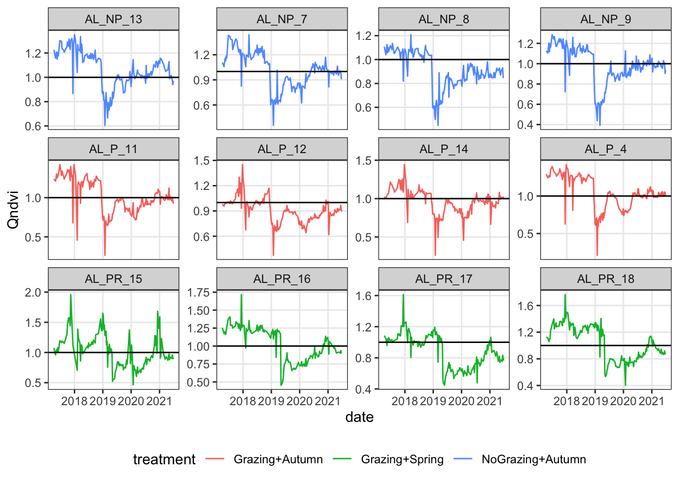
qndvi_avg <- qndvi_long %>%
  group_by(date, treatment) %>%
  summarise(mean = mean(Qndvi, na.rm=TRUE),
            sd = sd(Qndvi, na.rm=TRUE),
            se = plotrix::std.error(Qndvi, na.rm=TRUE))
qndvi_avg %>%
filter(treatment != "Grazing+Spring") %>%
ggplot(aes(x=date, y=mean, colour=treatment, fill=treatment)) +
geom_ribbon(aes(ymin = mean - se, ymax=mean+se), alpha = .3) +
geom_line(aes(y=mean)) +
theme_bw() +
theme(panel.grid.minor = element_blank()) +
geom_hline(yintercept = 1) +
scale_colour_manual(values=c("blue", "orange")) +
scale_fill_manual(values=c("blue", "orange")) library(dygraphs)
library(xts)
np <- qndvi_avg %>%
filter(treatment == "NoGrazing+Autumn") %>%
rowwise() %>%
mutate(lwr.np = mean - se,
upr.np = mean + se) %>%
dplyr::select(date, mean.np = mean, lwr.np, upr.np)
p <- qndvi_avg %>%
filter(treatment == "Grazing+Autumn") %>%
rowwise() %>%
mutate(lwr.p = mean - se,
upr.p = mean + se) %>%
dplyr::select(date, mean.p = mean, lwr.p, upr.p)
pr <- qndvi_avg %>%
filter(treatment == "Grazing+Spring") %>%
rowwise() %>%
mutate(lwr.pr = mean - se,
upr.pr = mean + se) %>%
dplyr::select(date, mean.pr = mean, lwr.pr, upr.pr)
df.ts <- inner_join(np, p) %>%
inner_join(pr)
ts <- xts(x= df.ts[,-1], order.by =df.ts$date)Grazing+Autumn vs. NoGrazing+Autumn
QNDVI
### NDVI
All series
QNDVI
NDVI
Appendix
- Explore NDVI evolution of control plots
control_np <- ndvi_avg %>%
  filter(str_detect(NOMBRE, "AL_CON_NP")) %>%
  group_by(date) %>%
  summarise(
    CONTROL = mean(ndvi_mean, na.rm = TRUE),
    CONTROL_sd = sd(ndvi_mean, na.rm = TRUE),
    CONTROL_se = plotrix::std.error(ndvi_mean, na.rm = TRUE),
    n = length(ndvi_mean)
  ) %>%
  ungroup()

control_p <- ndvi_avg %>%
  filter(str_detect(NOMBRE, "AL_CON_P")) %>%
  group_by(date) %>%
  summarise(
    CONTROL = mean(ndvi_mean, na.rm = TRUE),
    CONTROL_sd = sd(ndvi_mean, na.rm = TRUE),
    CONTROL_se = plotrix::std.error(ndvi_mean, na.rm = TRUE),
    n = length(ndvi_mean)
  ) %>%
  ungroup()

control_all <- ndvi_avg %>%
  filter(str_detect(NOMBRE, "AL_CON_")) %>%
  group_by(date) %>%
  summarise(
    CONTROL = mean(ndvi_mean, na.rm = TRUE),
    CONTROL_sd = sd(ndvi_mean, na.rm = TRUE),
    CONTROL_se = plotrix::std.error(ndvi_mean, na.rm = TRUE),
    n = length(ndvi_mean)
  ) %>%
  ungroup()
ggplot(control_all, aes(x=date, y=CONTROL))+
geom_line() +
geom_line(data=control_np, aes(x=date, y=CONTROL), colour = "blue") +
geom_line(data=control_p, aes(x=date, y=CONTROL), colour = "red") +
theme_bw() 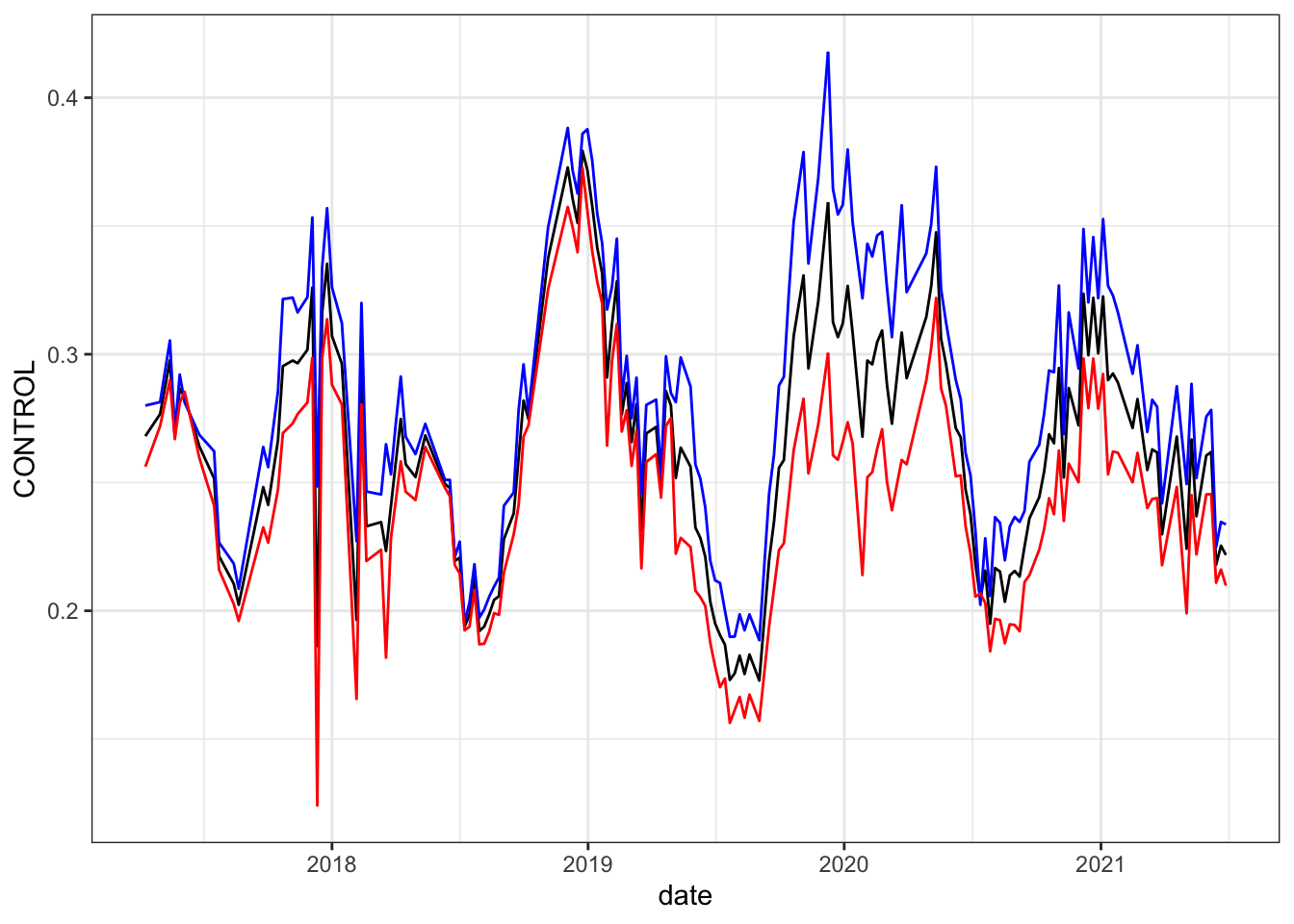
sessionInfo()R version 4.0.2 (2020-06-22)
Platform: x86_64-apple-darwin17.0 (64-bit)
Running under: macOS Catalina 10.15.3
Matrix products: default
BLAS: /Library/Frameworks/R.framework/Versions/4.0/Resources/lib/libRblas.dylib
LAPACK: /Library/Frameworks/R.framework/Versions/4.0/Resources/lib/libRlapack.dylib
locale:
[1] en_US.UTF-8/en_US.UTF-8/en_US.UTF-8/C/en_US.UTF-8/en_US.UTF-8
attached base packages:
[1] stats graphics grDevices utils datasets methods base
other attached packages:
[1] ISOweek_0.6-2 lubridate_1.7.10 xts_0.12.1 zoo_1.8-8
[5] dygraphs_1.1.1.6-1 plotrix_3.8-1 DiagrammeR_1.0.6.1 here_1.0.1
[9] forcats_0.5.1 stringr_1.4.0 dplyr_1.0.6 purrr_0.3.4
[13] readr_1.4.0 tidyr_1.1.3 tibble_3.1.2 ggplot2_3.3.3
[17] tidyverse_1.3.1 workflowr_1.6.2
loaded via a namespace (and not attached):
[1] Rcpp_1.0.6 lattice_0.20-41 visNetwork_2.0.9 assertthat_0.2.1
[5] rprojroot_2.0.2 digest_0.6.27 utf8_1.1.4 R6_2.5.0
[9] cellranger_1.1.0 backports_1.2.1 reprex_2.0.0 evaluate_0.14
[13] highr_0.8 httr_1.4.2 pillar_1.6.1 rlang_0.4.10
[17] readxl_1.3.1 rstudioapi_0.13 whisker_0.4 jquerylib_0.1.3
[21] rmarkdown_2.8 labeling_0.4.2 htmlwidgets_1.5.3 munsell_0.5.0
[25] broom_0.7.6 compiler_4.0.2 httpuv_1.5.5 modelr_0.1.8
[29] xfun_0.23 pkgconfig_2.0.3 htmltools_0.5.1.1 tidyselect_1.1.0
[33] fansi_0.4.2 crayon_1.4.1 dbplyr_2.1.1 withr_2.4.1
[37] later_1.1.0.1 grid_4.0.2 jsonlite_1.7.2 gtable_0.3.0
[41] lifecycle_1.0.0 DBI_1.1.1 git2r_0.28.0 magrittr_2.0.1
[45] scales_1.1.1 cli_2.5.0 stringi_1.5.3 farver_2.0.3
[49] fs_1.5.0 promises_1.2.0.1 xml2_1.3.2 bslib_0.2.4
[53] ellipsis_0.3.2 generics_0.1.0 vctrs_0.3.8 RColorBrewer_1.1-2
[57] tools_4.0.2 glue_1.4.2 hms_1.0.0 yaml_2.2.1
[61] colorspace_2.0-0 rvest_1.0.0 knitr_1.31 haven_2.3.1
[65] sass_0.3.1