Comparison drone_campo
2021-09-23
Last updated: 2021-10-26
Checks: 6 1
Knit directory:
dronveg_alcontar/
This reproducible R Markdown analysis was created with workflowr (version 1.6.2). The Checks tab describes the reproducibility checks that were applied when the results were created. The Past versions tab lists the development history.
The R Markdown file has unstaged changes.
To know which version of the R Markdown file created these
results, you’ll want to first commit it to the Git repo. If
you’re still working on the analysis, you can ignore this
warning. When you’re finished, you can run
wflow_publish to commit the R Markdown file and
build the HTML.
Great job! The global environment was empty. Objects defined in the global environment can affect the analysis in your R Markdown file in unknown ways. For reproduciblity it’s best to always run the code in an empty environment.
The command set.seed(20210923) was run prior to running the code in the R Markdown file.
Setting a seed ensures that any results that rely on randomness, e.g.
subsampling or permutations, are reproducible.
Great job! Recording the operating system, R version, and package versions is critical for reproducibility.
Nice! There were no cached chunks for this analysis, so you can be confident that you successfully produced the results during this run.
Great job! Using relative paths to the files within your workflowr project makes it easier to run your code on other machines.
Great! You are using Git for version control. Tracking code development and connecting the code version to the results is critical for reproducibility.
The results in this page were generated with repository version c72b76c. See the Past versions tab to see a history of the changes made to the R Markdown and HTML files.
Note that you need to be careful to ensure that all relevant files for the
analysis have been committed to Git prior to generating the results (you can
use wflow_publish or wflow_git_commit). workflowr only
checks the R Markdown file, but you know if there are other scripts or data
files that it depends on. Below is the status of the Git repository when the
results were generated:
Ignored files:
    Ignored:    .Rhistory
    Ignored:    .Rproj.user/

Untracked files:
    Untracked:  analysis/ecology-letters.csl
    Untracked:  analysis/references.bib

Unstaged changes:
    Modified:   analysis/compara_drone_campo.Rmd
Note that any generated files, e.g. HTML, png, CSS, etc., are not included in this status report because it is ok for generated content to have uncommitted changes.
These are the previous versions of the repository in which changes were made
to the R Markdown (analysis/compara_drone_campo.Rmd) and HTML (docs/compara_drone_campo.html)
files. If you’ve configured a remote Git repository (see
?wflow_git_remote), click on the hyperlinks in the table below to
view the files as they were in that past version.
| File | Version | Author | Date | Message |
|---|---|---|---|---|
| html | a6013e7 | ajpelu | 2021-09-30 | Build site. |
| Rmd | 5160f1b | ajpelu | 2021-09-30 | add rms table |
| html | 23681f5 | ajpelu | 2021-09-30 | Build site. |
| Rmd | 2c0f184 | ajpelu | 2021-09-30 | wflow_publish(“analysis/compara_drone_campo.Rmd”) |
0.1 Introduction
- Read and prepare data
Summary of the analysis:
Two drone methods (TODO: Document):
- AREA_VEG_m2 rename as cov.drone1
- COBERTURA rename as cov.drone2
Ground-field coverage measures (COB_TOTAL_M2), rename as cov.campo
Explore by coverage class.
Another variables to consider:
- Shannon diversity index
- Phytovolumen (m^3/ha)
- Richness
- Slope (derived of DEM from drone)
1 Plant coverage
- Compare Drone vs Ground field measurement
1.1 Which method of the plant coverage estimation by drones should be used?
We use two methods of drone measurement (TODO: Document)
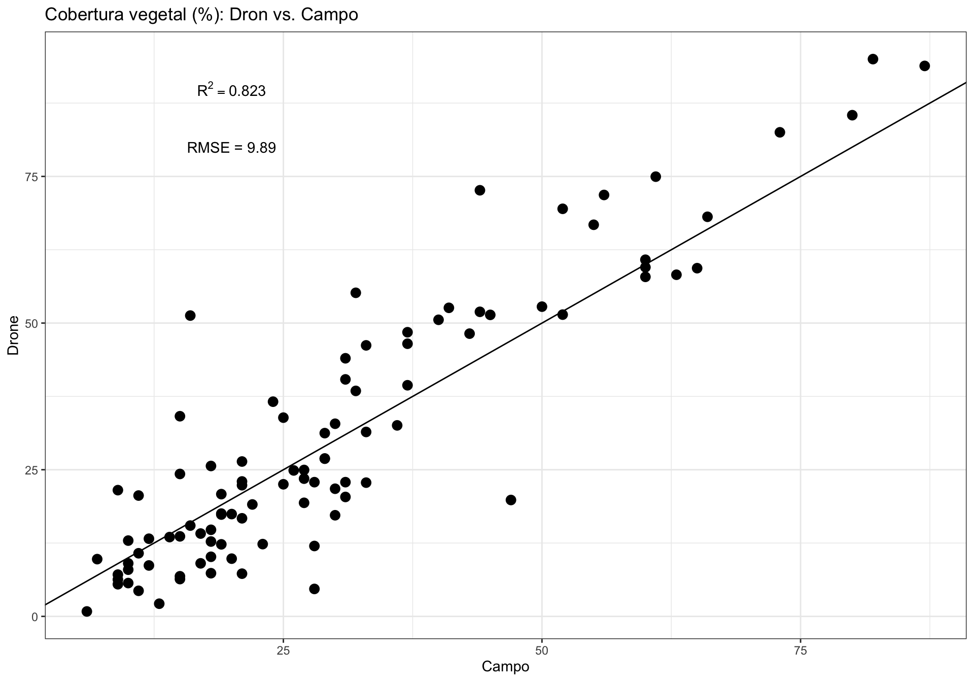
First, we compare the correlation between the coverage measurement derived from each drone approach (drone), and the ground field measurement (campo).
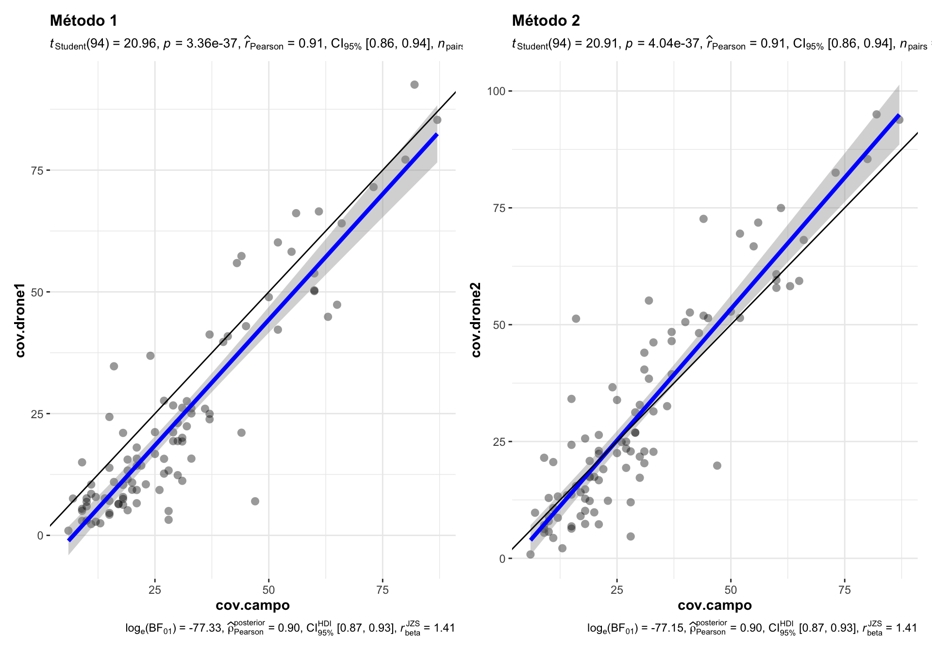
Figure 1.1: Comparison of the correlation between drone-field ground coverage measurement using two different drone-coverage approaches.
| Version | Author | Date |
|---|---|---|
| 23681f5 | ajpelu | 2021-09-30 |
Correlations between drone vs. campo measurement yielded high and significant pearson values (\(R^2=\) 0.91, p-values < 0.001 in both cases).
The method 1 (cov.drone1) show underestimate values of the perfect adjust, i.e. the estimation of coverage by drone is lower (for most of the measurements) than the ground-field coverage estimation (Figure 1.1). This uderestimation occurs along the all interval of coverage values.
On the other hand, the method 2, show closer values to the perfect line, overall at lower coverage values (up to 30 %). A slight overstimate is observed for values greather than 50 % (Figure 1.1).
Conclusion: We selected the method 2 (TODO document)
1.2 Explore correlations conditionally to vegetation cover (RANGO_INFOCA).
There are four categories of plant coverage (coverage class):
- Matorral claro (<25%) (RANGO_INFOCA = 1)
- Matorral medio (25-50%) (RANGO_INFOCA = 2)
- Espartal denso (>75%) (RANGO_INFOCA = 3)
- Aulagar denso (>75%) (RANGO_INFOCA = 4)
We explore the correlation bewteen drone-field measurement for each of the coverage class. We use the RMSE (Root Mean Squared Error) to explore the accuracy of the correlations for each coverage class. The RMSE is a measure of the accuracy, and here it is used to compare the errors of the correlation for each of the coverage class. RMSE is scale-dependent, but we don’t have this problem in our models (all are in the same sclaes, i.e. percentage). Lower values indicates better fit.
| cover class | RMSE | min. | max. | norm. RMSE % |
|---|---|---|---|---|
| Aulagar denso (>75%) | 12.69 | 10 | 61 | 24.89 |
| Espartal denso (>75%) | 7.63 | 9 | 87 | 9.78 |
| Matorral claro (<25%) | 7.30 | 6 | 28 | 33.18 |
| Matorral medio (25-50%) | 10.89 | 9 | 63 | 20.16 |
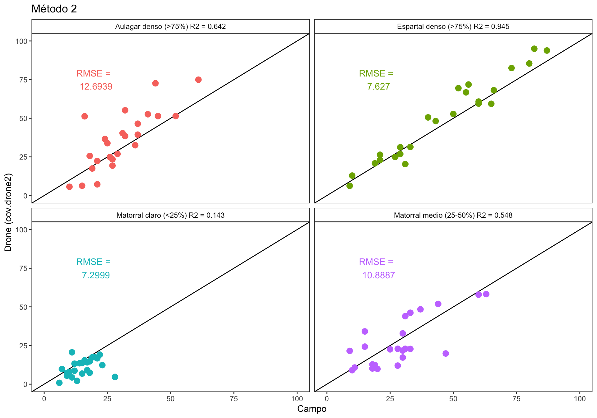
Figure 1.2: Correlation between drone vs. field plant coverage measurement. Each panel show the correlation by coverage classes.
| Version | Author | Date |
|---|---|---|
| 23681f5 | ajpelu | 2021-09-30 |
- We can see in the Figure 1.2, that the lower RMSE values are yielded by the coverage classes “Matorral claro (<25%)” and “Espartal denso (>75%)” with 7.29 and 7.62 % of the error respectively.
2 Correlation vs Other variables
Is there any relationship between correlation and other variables?. We could be interested to explore how other variables could influence the drone-field correlation, e.g. the richness or the slope. Several approaches can be used (exploratory analysis, residuals, etc.)
- Compute residuals and absolute residuals
m <- lm(cov.drone2 ~ cov.campo, data=df)
df <- df %>% modelr::add_residuals(m) %>%
  mutate(resid.abs = abs(resid))
2.1 Shannon diversity
We explore if the Shannon diversity of each plot does influence the correlation between drone-field measurement. Two approaches were carried out: - Is there any relation of the drone-field residuals and the Shannon diversity. For instance, if higher residual values (absolute values) will correspond with higher shannon diversity values, then we could state that the higher the shannon diversity the lower the accuracy of the correlation between drone-field measurment.
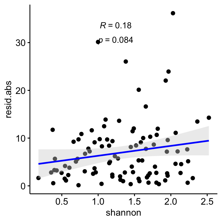
Figure 2.1: Relation between the correlation residuals (drone-field correlation) and the Shannon diversity index (H’). Residulas are shown in absolute values.
| Version | Author | Date |
|---|---|---|
| 23681f5 | ajpelu | 2021-09-30 |
As we can see in Figure 2.1, there in no significant pattern for the relation of Shannon index and residuals, so the correlation between drone and field coverage seems not to be influenced by the Shannon diversity. However, we observed that the plots with higher Shannon diversity values are those with coverage values below 25 % (see Figure 2.2)
Figure 2.2: Correlation between drone vs. field plant coverage measurement. Size and colour points indicates Shannon diversity values
In this sense, we also could be interested in the relationship between each of the coverage measurement (drone or field-measurement) and the Shannon diversity. For this purpose, we fitted a Non-Linear Squares curve for each of the measurement. The curve takes the form: \[Shannon = a\times\exp^{-b \times Coverage}\]
As, we can see in the Figure 2.3, there is a decay relationships between Shannon diversity values and the coverage estimated by drone (\(R_{Nagelk.}^2 =\) 0.313), or by field (\(R_{Nagelk.}^2 =\) 0.398).
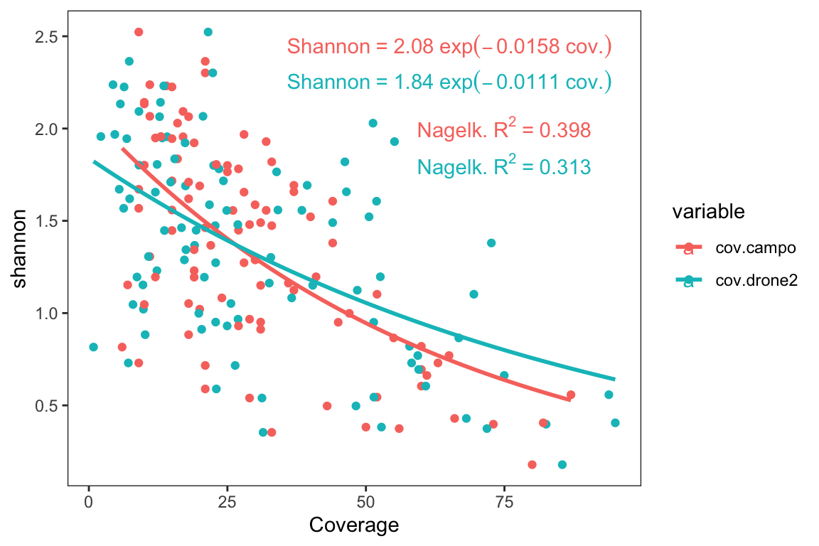
Figure 2.3: Non-linear relation between Shannon index and drone- (blue) and field- (pink) plant coverage
| Version | Author | Date |
|---|---|---|
| 23681f5 | ajpelu | 2021-09-30 |
# A tibble: 2 x 4
  variable   r_square     a      b
  <chr>         <dbl> <dbl>  <dbl>
1 cov.campo     0.398  2.08 0.0158
2 cov.drone2    0.313  1.84 0.0111
2.2 Richness
Similarly to Shannon, we explore relationship between Richness and residulas. We find a positive relationships between the residuals and the richness, so the plot showing higher residual values seem to be those with higher richness (Figure 2.4). However we didn’t find relation between richness and coverage (see Figure 2.4).
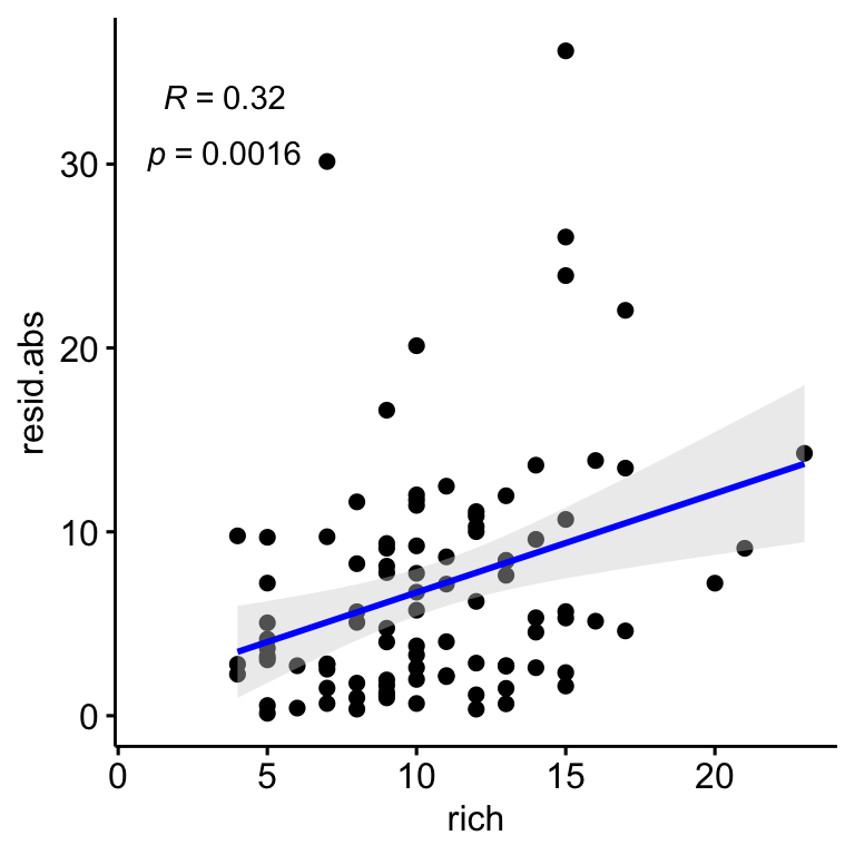
Figure 2.4: Relation between the correlation residuals (drone-field correlation) and the Richness. Residulas are shown in absolute values.
| Version | Author | Date |
|---|---|---|
| 23681f5 | ajpelu | 2021-09-30 |
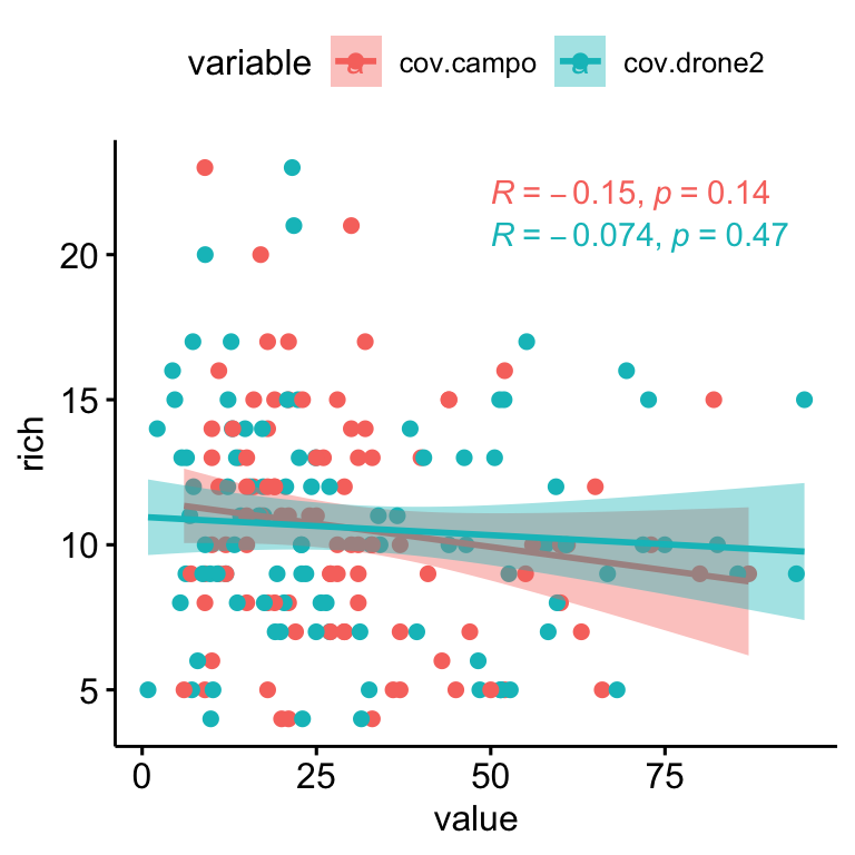
Figure 2.5: Relation between Richness and drone- (blue) and field- (pink) plant coverage.
| Version | Author | Date |
|---|---|---|
| 23681f5 | ajpelu | 2021-09-30 |
Figure 2.6: Correlation between drone vs. field plant coverage measurement. Size and colour points indicates Richness values
2.3 Slope
We find no significant relationships between the residuals (absolute values) and the slope (\(R^2\) = 0.0047, p-value = 0.506; Figure 2.7); and there are not also relationship of slope and plant coverages (see Figure 2.8).
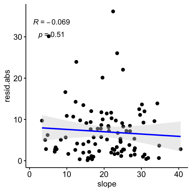
Figure 2.7: Relation between the correlation residuals (drone-field correlation) and the Slope, Residulas are shown in absolute values.
| Version | Author | Date |
|---|---|---|
| 23681f5 | ajpelu | 2021-09-30 |
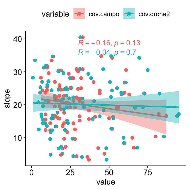
Figure 2.8: Relation between Slope and drone- (blue) and field- (pink) plant coverage
| Version | Author | Date |
|---|---|---|
| 23681f5 | ajpelu | 2021-09-30 |
3 Relation with composition
We also want to explore if the species composition affects to the correlation bewteen coverages. For instance, are the plots with dominance of certain species showing higher values of correlation residuals? or is the correlation bewteen coverages (drone vs. field) worse at plots with a given species composition?
For this purpose our approach were:
Generate an ordination plot of the field plots according their species composition. We used non-Metric Multidimensional Scaling method (NMDS) with three axis.
Then we fitted surface responses of our variable of interest (absolute residuals)
3.1 NMDS Results
- Compute NMDS
Square root transformation
Wisconsin double standardization
Run 0 stress 0.1863478
Run 1 stress 0.1860835
... New best solution
... Procrustes: rmse 0.008266918  max resid 0.04977916
Run 2 stress 0.1887491
Run 3 stress 0.1899427
Run 4 stress 0.1862349
... Procrustes: rmse 0.02180245  max resid 0.1574149
Run 5 stress 0.1869263
Run 6 stress 0.1871034
Run 7 stress 0.1870711
Run 8 stress 0.1860625
... New best solution
... Procrustes: rmse 0.002889091  max resid 0.01335322
Run 9 stress 0.1886365
Run 10 stress 0.1891944
Run 11 stress 0.1868303
Run 12 stress 0.1860739
... Procrustes: rmse 0.001265871  max resid 0.009556574
... Similar to previous best
Run 13 stress 0.18908
Run 14 stress 0.1868857
Run 15 stress 0.188423
Run 16 stress 0.1860552
... New best solution
... Procrustes: rmse 0.01682101  max resid 0.1538522
Run 17 stress 0.1890815
Run 18 stress 0.1870701
Run 19 stress 0.1868194
Run 20 stress 0.18732
Run 21 stress 0.1894233
Run 22 stress 0.1860623
... Procrustes: rmse 0.01682793  max resid 0.1536885
Run 23 stress 0.186336
... Procrustes: rmse 0.01845432  max resid 0.1552014
Run 24 stress 0.187697
Run 25 stress 0.1868292
Run 26 stress 0.1866867
Run 27 stress 0.1870719
Run 28 stress 0.1899394
Run 29 stress 0.1876515
Run 30 stress 0.1864186
... Procrustes: rmse 0.02085871  max resid 0.1592674
*** No convergence -- monoMDS stopping criteria:
    11: no. of iterations >= maxit
    19: stress ratio > sratmax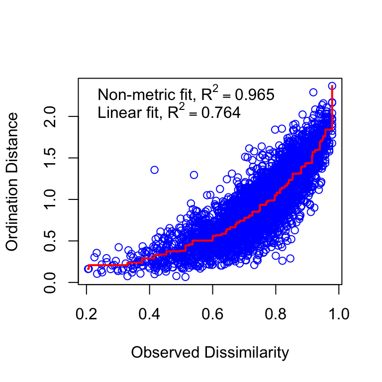
Figure 3.1: NMDS stressplot
| Version | Author | Date |
|---|---|---|
| 23681f5 | ajpelu | 2021-09-30 |
## Vectores
set.seed(123)
ef <- envfit(nmds3, dfnmds$resid.abs, choices=1:3, perm = 1000)
ef
***VECTORS

        NMDS1    NMDS2    NMDS3     r2 Pr(>r)
[1,]  0.96095 -0.25532 -0.10674 0.0359 0.3407
Permutation: free
Number of permutations: 1000
# Surface responses
or <- ordisurf(nmds3, dfnmds$resid.abs, add=F)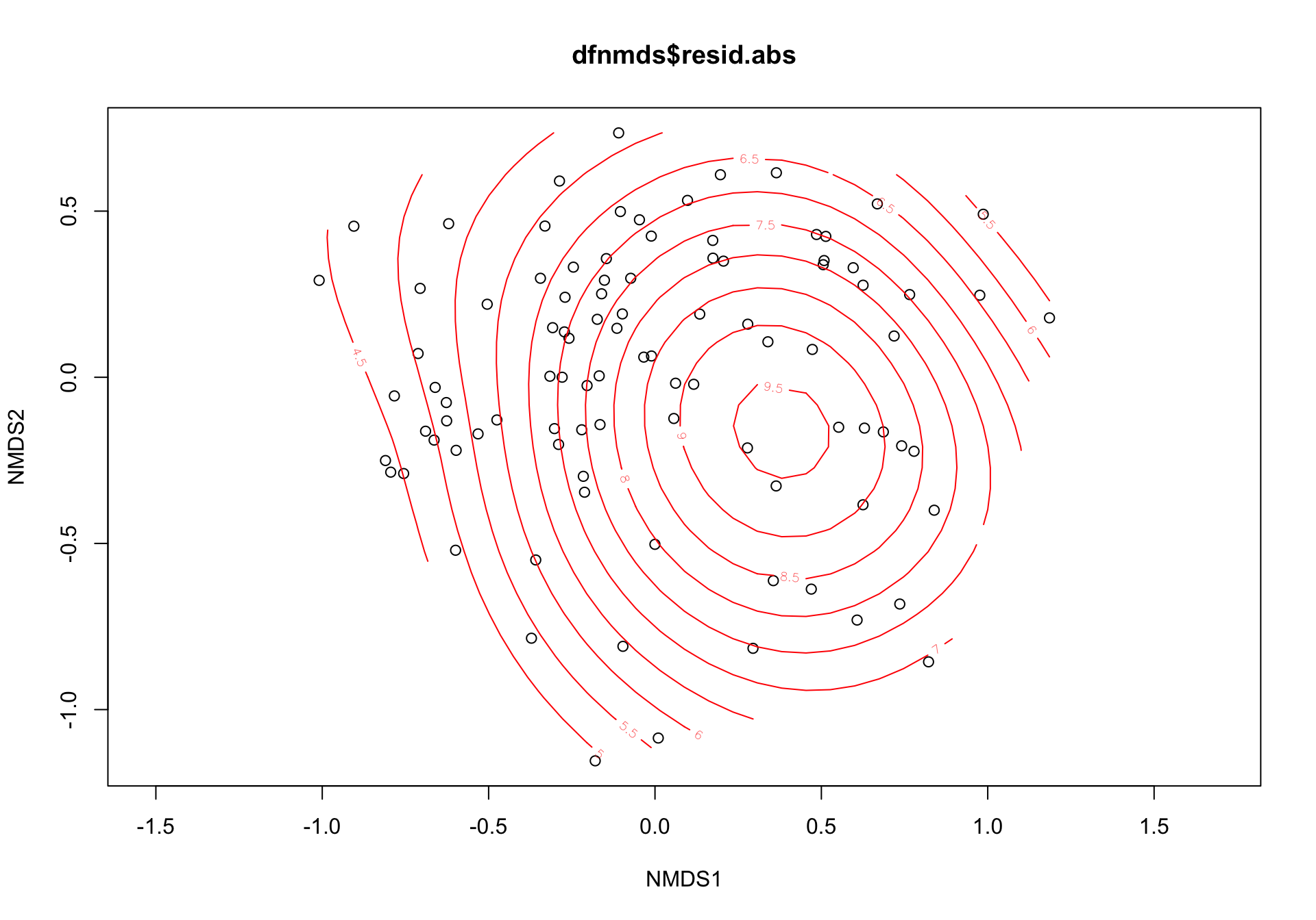
| Version | Author | Date |
|---|---|---|
| a6013e7 | ajpelu | 2021-09-30 |
s_or <- summary(or)

# Estadístico
s_or$s.table[,"F"]
[1] 0.8604552# r2 ajustada
s_or$r.sq[1] 0.07536934# p-value de la superficie ajustada
s_or$s.table[,"p-value"][1] 0.03093265# Devianza explicada
s_or$dev.expl[1] 0.1057318We observed an acceptable ordination plot (stress valor < 0.2) (3.1). The surface response of the residuals over this ordination plot was poor and not significant (\(R^2\) = 0.08, p.value = 0.0309) (see Figure 3.2)
Family: gaussian
Link function: identity

Formula:
y ~ s(x1, x2, k = 10, bs = "tp", fx = FALSE)

Estimated degrees of freedom:
3.12  total = 4.12

REML score: 314.4757 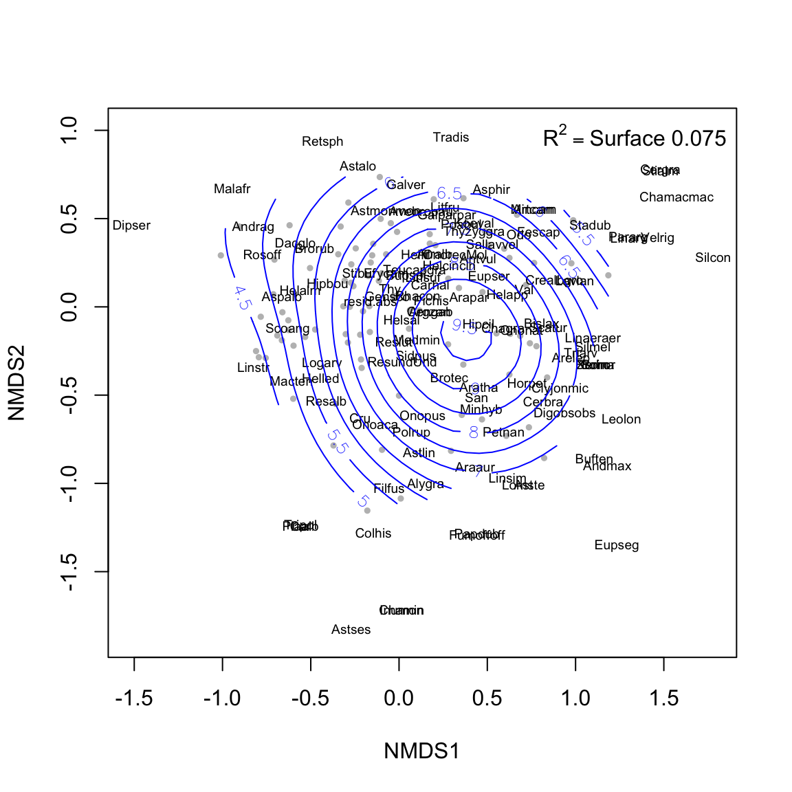
Figure 3.2: Ordination plot of the species composition (label = species; red points = sites) and surface response of the residuals (absolute values)
| Version | Author | Date |
|---|---|---|
| 23681f5 | ajpelu | 2021-09-30 |
3.1.1 Another plots
3.1.2 Notas
Aplicar análisis de clasificación (\(\kappa\) coefficient). Ver un ejemplo en Cunliffe et al. (2016).
Revisar trabajos de Cunliffe et al. (2016), Abdullah et al. (2021) y similares.
4 References
R version 4.0.2 (2020-06-22)
Platform: x86_64-apple-darwin17.0 (64-bit)
Running under: macOS Catalina 10.15.3

Matrix products: default
BLAS:   /Library/Frameworks/R.framework/Versions/4.0/Resources/lib/libRblas.dylib
LAPACK: /Library/Frameworks/R.framework/Versions/4.0/Resources/lib/libRlapack.dylib

locale:
[1] en_US.UTF-8/en_US.UTF-8/en_US.UTF-8/C/en_US.UTF-8/en_US.UTF-8

attached base packages:
[1] stats     graphics  grDevices utils     datasets  methods   base

other attached packages:
 [1] vegan_2.5-7        lattice_0.20-41    permute_0.9-5      ggpubr_0.4.0
 [5] fuzzySim_3.0       ggpmisc_0.3.9      workflowsets_0.1.0 workflows_0.2.3
 [9] tune_0.1.6         rsample_0.1.0      recipes_0.1.16     parsnip_0.1.7
[13] modeldata_0.1.1    infer_1.0.0        dials_0.0.10       scales_1.1.1.9000
[17] tidymodels_0.1.3   broom_0.7.9        kableExtra_1.3.1   nlstools_1.0-2
[21] sjPlot_2.8.9       modelr_0.1.8       Metrics_0.1.4      yardstick_0.0.8
[25] ggiraph_0.7.10     cowplot_1.1.1      patchwork_1.1.1    ggstatsplot_0.7.2
[29] plotly_4.9.3       DT_0.17            plotrix_3.8-1      readxl_1.3.1
[33] forcats_0.5.1      stringr_1.4.0      dplyr_1.0.6        purrr_0.3.4
[37] readr_1.4.0        tidyr_1.1.3        tibble_3.1.2       ggplot2_3.3.5
[41] tidyverse_1.3.1    here_1.0.1

loaded via a namespace (and not attached):
  [1] estimability_1.3          coda_0.19-4
  [3] knitr_1.31                multcomp_1.4-16
  [5] data.table_1.14.0         rpart_4.1-15
  [7] hardhat_0.1.6             generics_0.1.0
  [9] GPfit_1.0-8               TH.data_1.0-10
 [11] future_1.21.0             correlation_0.6.1
 [13] webshot_0.5.2             xml2_1.3.2
 [15] lubridate_1.7.10          httpuv_1.5.5
 [17] assertthat_0.2.1          gower_0.2.2
 [19] WRS2_1.1-1                xfun_0.23
 [21] hms_1.0.0                 jquerylib_0.1.3
 [23] evaluate_0.14             promises_1.2.0.1
 [25] fansi_0.4.2               dbplyr_2.1.1
 [27] DBI_1.1.1                 htmlwidgets_1.5.3
 [29] reshape_0.8.8             kSamples_1.2-9
 [31] Rmpfr_0.8-2               paletteer_1.3.0
 [33] ellipsis_0.3.2            backports_1.2.1
 [35] bookdown_0.21.6           insight_0.14.4
 [37] ggcorrplot_0.1.3          vctrs_0.3.8
 [39] sjlabelled_1.1.7          abind_1.4-5
 [41] cachem_1.0.4              withr_2.4.1
 [43] emmeans_1.5.4             cluster_2.1.0
 [45] lazyeval_0.2.2            crayon_1.4.1
 [47] pkgconfig_2.0.3           SuppDists_1.1-9.5
 [49] labeling_0.4.2            nlme_3.1-152
 [51] statsExpressions_1.1.0    nnet_7.3-15
 [53] rlang_0.4.12              globals_0.14.0
 [55] lifecycle_1.0.1           MatrixModels_0.4-1
 [57] sandwich_3.0-0            cellranger_1.1.0
 [59] rprojroot_2.0.2           datawizard_0.2.0.1
 [61] Matrix_1.3-2              mc2d_0.1-18
 [63] carData_3.0-4             boot_1.3-26
 [65] zoo_1.8-8                 reprex_2.0.0
 [67] whisker_0.4               viridisLite_0.4.0
 [69] PMCMRplus_1.9.0           parameters_0.14.0
 [71] pROC_1.17.0.1             workflowr_1.6.2
 [73] multcompView_0.1-8        parallelly_1.24.0
 [75] rstatix_0.6.0             ggeffects_1.0.1
 [77] ggsignif_0.6.0            memoise_2.0.0
 [79] magrittr_2.0.1            plyr_1.8.6
 [81] compiler_4.0.2            lme4_1.1-27.1
 [83] cli_2.5.0                 DiceDesign_1.9
 [85] listenv_0.8.0             pbapply_1.4-3
 [87] MASS_7.3-53               mgcv_1.8-33
 [89] tidyselect_1.1.1          stringi_1.7.4
 [91] highr_0.8                 yaml_2.2.1
 [93] ggrepel_0.9.1             grid_4.0.2
 [95] sass_0.3.1                tools_4.0.2
 [97] parallel_4.0.2            rio_0.5.16
 [99] rstudioapi_0.13           uuid_0.1-4
[101] foreach_1.5.1             foreign_0.8-81
[103] git2r_0.28.0              ipmisc_5.0.2
[105] prodlim_2019.11.13        pairwiseComparisons_3.1.3
[107] farver_2.1.0              digest_0.6.27
[109] lava_1.6.8.1              BWStest_0.2.2
[111] Rcpp_1.0.7                car_3.0-10
[113] BayesFactor_0.9.12-4.2    performance_0.7.2
[115] later_1.1.0.1             httr_1.4.2
[117] effectsize_0.4.5          sjstats_0.18.1
[119] colorspace_2.0-2          rvest_1.0.0
[121] fs_1.5.0                  splines_4.0.2
[123] rematch2_2.1.2            systemfonts_1.0.0
[125] xtable_1.8-4              gmp_0.6-2
[127] jsonlite_1.7.2            nloptr_1.2.2.2
[129] timeDate_3043.102         zeallot_0.1.0
[131] ipred_0.9-9               R6_2.5.1
[133] lhs_1.1.3                 pillar_1.6.1
[135] htmltools_0.5.2           glue_1.4.2
[137] fastmap_1.1.0             minqa_1.2.4
[139] class_7.3-18              codetools_0.2-18
[141] mvtnorm_1.1-1             furrr_0.2.2
[143] utf8_1.1.4                bslib_0.2.4
[145] curl_4.3                  gtools_3.8.2
[147] zip_2.1.1                 openxlsx_4.2.3
[149] survival_3.2-7            rmarkdown_2.8
[151] munsell_0.5.0             iterators_1.0.13
[153] sjmisc_2.8.6              haven_2.3.1
[155] gtable_0.3.0              bayestestR_0.9.0